Customizing ggplot2 color and fill scales

Whenever we map color or fill as an aesthetic, ggplot2 uses a default color scheme, known as the color or fill scales in the grammar of graphics.

If you do not want to use the default color/fill scales, you can override the defaults by providing a different scale. This tutorial introduces some commonly-used scales which are accessible with ggplot2, including several popular scales from colorbrewer (a set of color scales originally devised for maps) and viridis (a set of color scales developed for plotting purposes).

Functions we can use to change the default color/fill scales include the following:

Mapped data type	Scale type	ggplot2 function
Discrete	colorbrewer	scale_<color/fill>_brewer(palette = 'name of palette')
Continuous	colorbrewer	scale_<color/fill>_distiller(palette = 'name of palette')
Discrete	viridis	scale_<color/fill>_viridis_d(option = 'name of palette')
Continuous	viridis	scale_<color/fill>_viridis_c(option = 'name of palette')
Discrete	Custom fills/colors	scale_<color/fill>_manual(values = c('array', 'of', 'colors', 'to', 'use'))
Continuous	Sequential gradient of custom fills/colors	scale_<color/fill>_gradient(low = 'low color', high = 'high color')
Continuous	Diverging gradient of custom fills/colors	scale_<color/fill>_gradient2(low = 'low color', high = 'high color', mid = 'mid color', midpoint = 'number')

The colorbrewer and viridis palettes

Below are the names and colors associated with colorbrewer (left) and viridis (right) palettes. Many, but not all, of these palettes are so-called “colorblind friendly,” meaning individuals with color vision deficiencies are still able to distinguish among the palette’s colors.

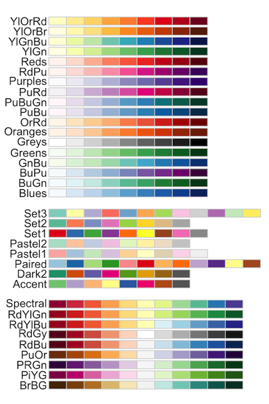
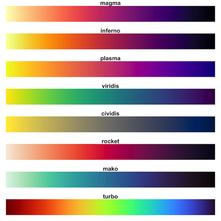
All colorbrewer palettes can be used for discrete data, but the middle set of palettes (Set3 through Accent) can not be used for continuous data. All viridis palettes can be used for both discrete and continuous data.

Examples

All examples shown here are made from a modified version of the msleep dataset with certain NA values removed (see below). Examples modify the default colors/fills of one of these plots, all of which use the default ggplot2 scales. We will also set the theme for all plots to include the legend on the bottom, for easier viewing in examples (learn more about that here)!

# Remove NAs from the columns awake, sleep_rem, and vore for plotting demonstration
# We'll call this dataset `msleep_clean`
msleep %>%
  tidyr::drop_na(awake, sleep_rem, vore) -> msleep_clean
  
# Set the plotting theme to place legends below plots
theme_set(theme(legend.position = "bottom"))

# First plot used in examples. Uses discrete color mapping.
ggplot(msleep_clean) + 
  aes(x = awake, 
      y = sleep_rem, 
      color = vore) + 
  geom_point() -> plot1

# Second plot used in examples. Uses discrete fill mapping.
ggplot(msleep_clean) + 
  aes(x = vore, 
      y = awake,
      fill = vore) + 
  geom_boxplot() -> plot2

# Third plot used in examples. Uses continuous color mapping.
ggplot(msleep_clean) + 
  aes(x = awake, 
      y = sleep_rem, 
      color = awake) + 
  geom_point() -> plot3

# Add plots together, which is allowed when you load the {patchwork} library
plot1 + plot2 + plot3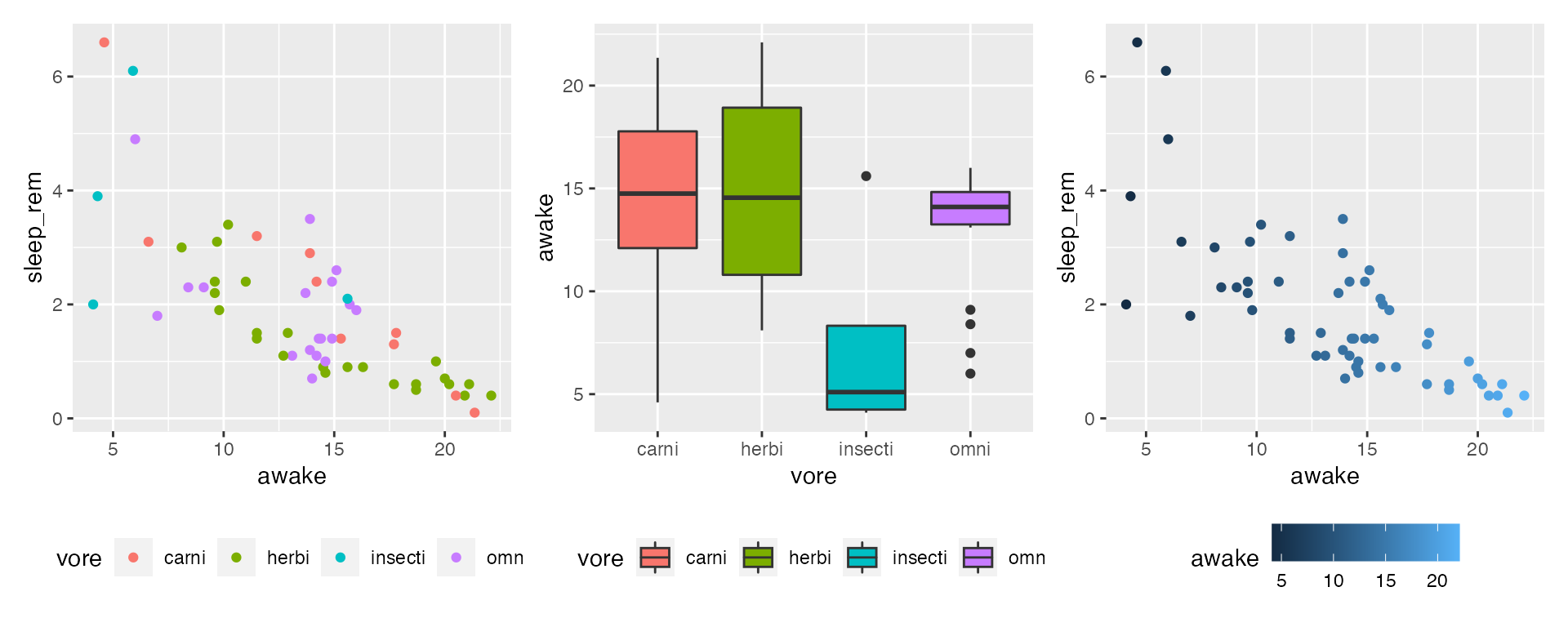

Customizing discrete data color/fill mappings

Using a custom scale

To create your own discrete palette, use the function scale_<color/fill>_manual(). Always make sure to use the right function name for the aesthetic you are considering. In other words, use scale_color_manual() to customize a color mapping, not to customize a fill mapping.

# Specify custom _colors_ for each vore category
ggplot(msleep_clean) + 
  aes(x = awake, 
      y = sleep_rem, 
      color = vore) + 
  geom_point() +
  scale_color_manual(values = c("blue", "orange", "magenta", "yellow"))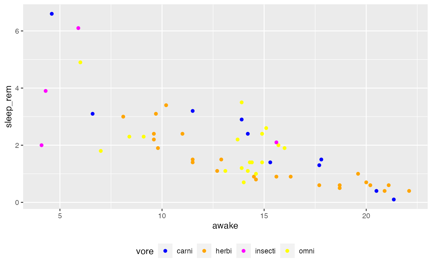

# Specify custom _fills_ for each vore category
ggplot(msleep_clean) + 
  aes(x = vore, 
      y = awake, 
      fill = vore) + 
  geom_boxplot() +
  scale_fill_manual(values = c("blue", "orange", "magenta", "yellow"))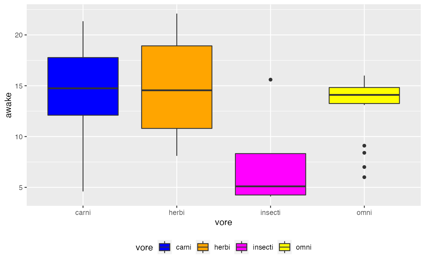

Using a colorbrewer scale

To use a colorbrewer palette with discrete data, use the function scale_<color/fill>_brewer() with the argument palette to specify which palette you want to use. Again, always make sure to use the right function name for the aesthetic you are considering. In other words, use scale_color_brewer() to customize a color mapping, not to customize a fill mapping.

# Specify custom _colors_ for each vore category
ggplot(msleep_clean) + 
  aes(x = awake, 
      y = sleep_rem, 
      color = vore) + 
  geom_point() +
  scale_color_brewer(palette = "Greens")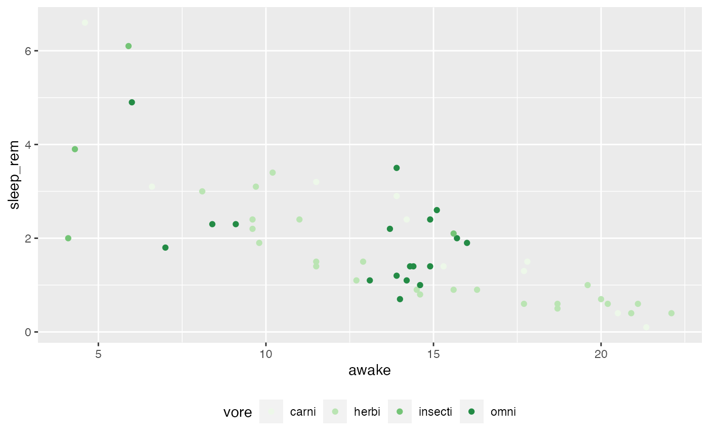

# Specify custom _fills_ for each vore category
ggplot(msleep_clean) + 
  aes(x = vore, 
      y = awake, 
      fill = vore) + 
  geom_boxplot() +
  # yellow --> green palette
  scale_fill_brewer(palette = "YlGn")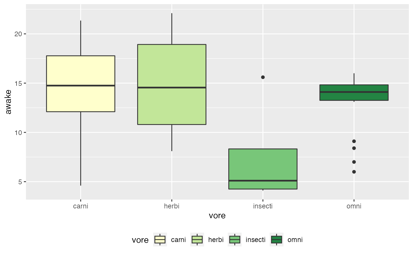

# You can reverse the order of the palette with `direction = -1`
# This argument works with any brewer function
ggplot(msleep_clean) + 
  aes(x = vore, 
      y = awake, 
      fill = vore) + 
  geom_boxplot() +
  # Switch palette direction 
  scale_fill_brewer(palette = "YlGn", 
                    direction = -1)

Using a viridis scale

To use a viridis palette with discrete data, use the function scale_<color/fill>_viridis_d() (d for discrete!) with the argument option (not palette) to specify which palette you want to use. Again, always make sure to use the right function name for the aesthetic you are considering. In other words, use scale_color_viridis_d() to customize a color mapping, not to customize a fill mapping.

# Specify custom _colors_ for each vore category
ggplot(msleep_clean) + 
  aes(x = awake, 
      y = sleep_rem, 
      color = vore) + 
  geom_point() +
  scale_color_viridis_d(option = "inferno")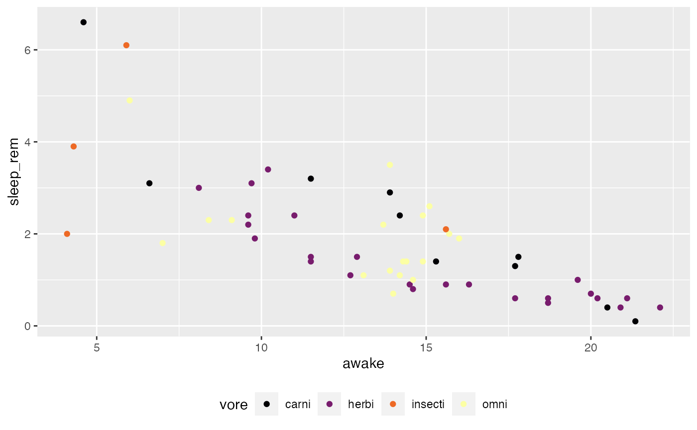

# Specify custom _colors_ for each vore category
ggplot(msleep_clean) + 
  aes(x = awake, 
      y = sleep_rem, 
      color = vore) + 
  geom_point() +
  # without `option`, the default viridis palette is used
  scale_color_viridis_d()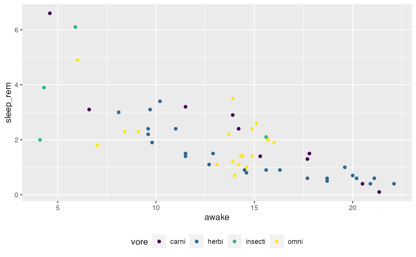

# You can reverse the order of the palette with `direction = -1`
# This argument works with any viridis function
ggplot(msleep_clean) + 
  aes(x = awake, 
      y = sleep_rem, 
      color = vore) + 
  geom_point() +
  # reverse the order of the palette
  scale_color_viridis_d(direction = -1)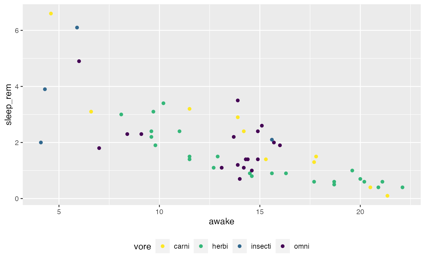

# Specify custom _fills_ for each vore category
ggplot(msleep_clean) + 
  aes(x = vore, 
      y = awake, 
      fill = vore) + 
  geom_boxplot() +
  scale_fill_viridis_d(option = "plasma")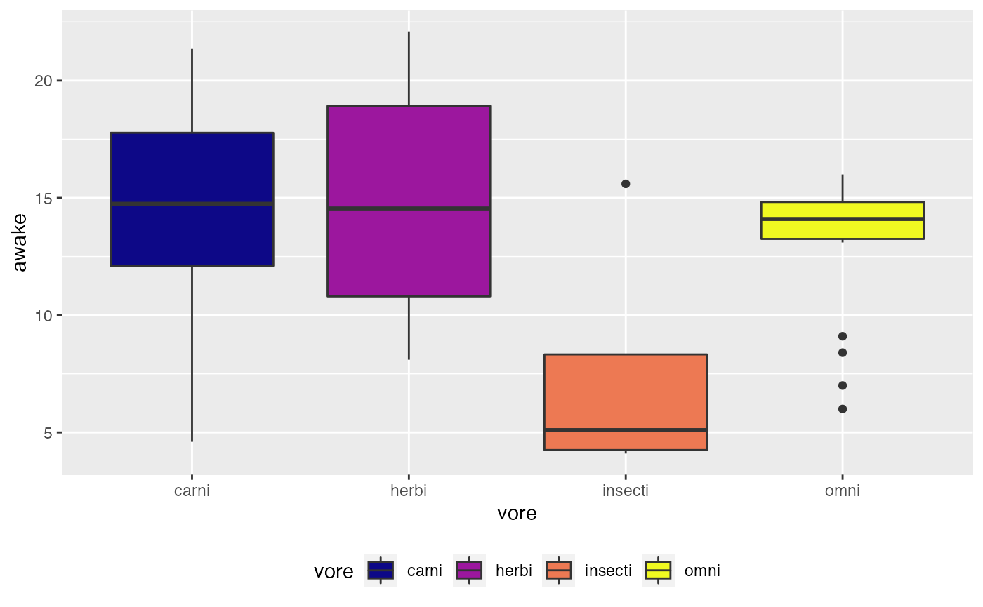

Customizing continuous data color/fill mappings

Using a custom scale

To create your own continuous palette, i.e. gradient, use either of these functions: + scale_<color/fill>_gradient(): A gradient from one color to another + scale_<color/fill>_gradient2(): A gradient from one color to another, with another color in the middle

# Specify a custom gradient for each value of awake, a continuous variable
ggplot(msleep_clean) + 
  aes(x = awake, 
      y = sleep_rem, 
      color = awake) + # Color is mapped to a continuous variable 
  geom_point() +
  # Gradient goes low-->high values, blue-->orange
  scale_color_gradient(low = "blue", high = "orange")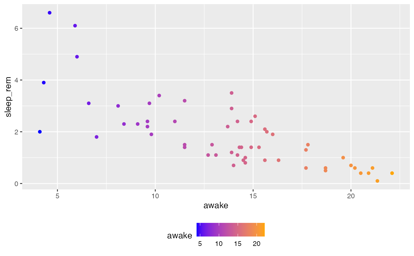

# Change the direction of your custom palette by switching low/high values
ggplot(msleep_clean) + 
  aes(x = awake, 
      y = sleep_rem, 
      color = awake) + # Color is mapped to a continuous variable 
  geom_point() +
  # Gradient goes low-->high values, blue-->orange
  scale_color_gradient(low = "orange", high = "blue")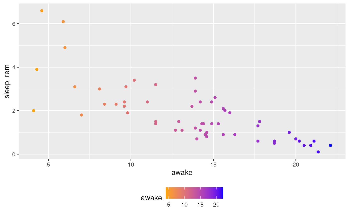

# Specify a custom gradient2 for each value of awake, a continuous variable
# BUT! The default midpoint "switch" is 0, and all awake values are _above 0_, so we see no gradient2
ggplot(msleep_clean) + 
  aes(x = awake, 
      y = sleep_rem, 
      color = awake) + # Color is mapped to a continuous variable 
  geom_point() +
  # Gradient goes low-->middle-->high values, blue-->black-->orange
  scale_color_gradient2(low = "blue", 
                        high = "orange", 
                        mid = "black")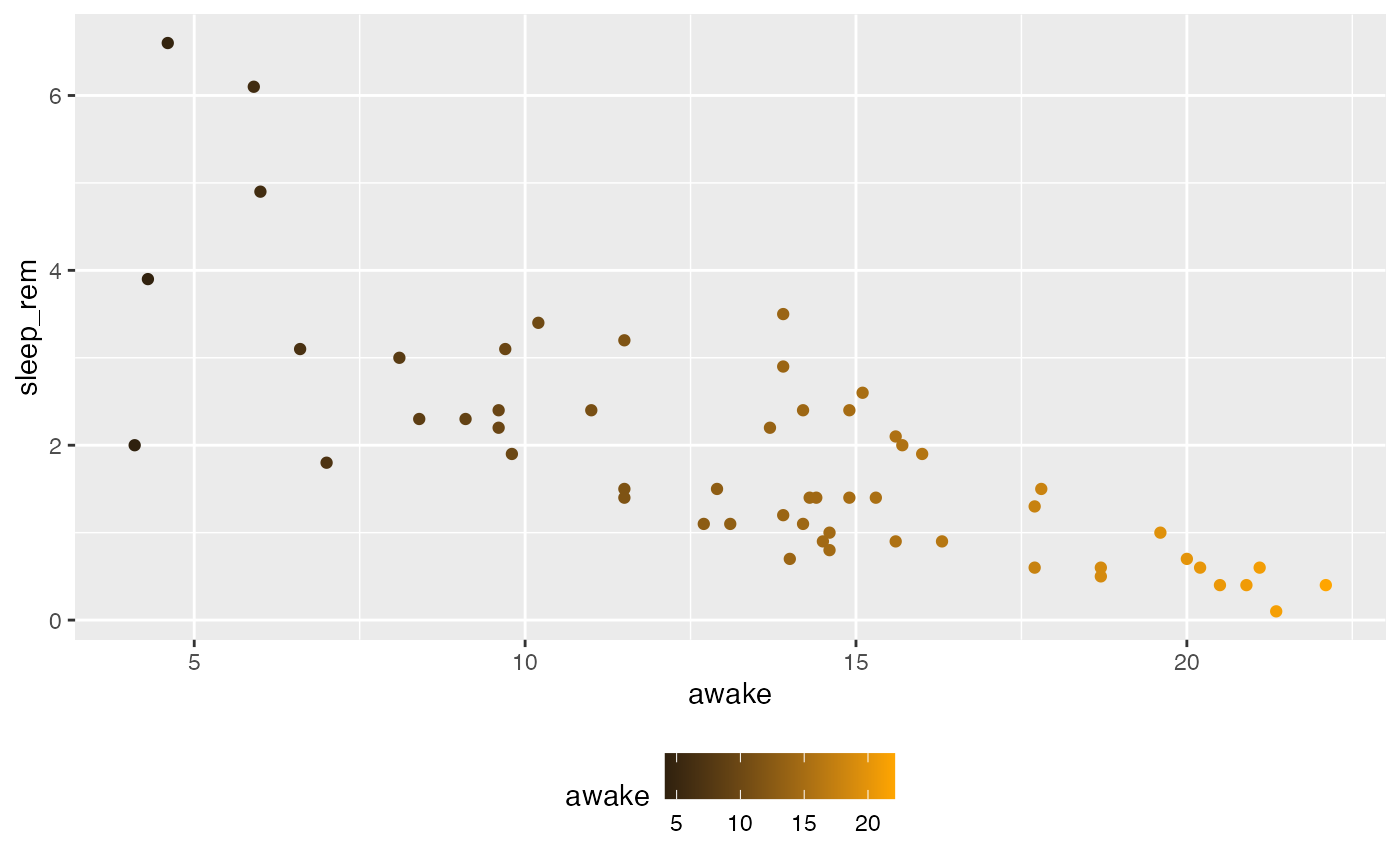

# Make the previous example "switch" the gradient2 at a midpoint of 13, for example
ggplot(msleep_clean) + 
  aes(x = awake, 
      y = sleep_rem, 
      color = awake) + # Color is mapped to a continuous variable 
  geom_point() +
  # Gradient goes low-->middle-->high values, blue-->black-->orange
  scale_color_gradient2(low = "blue", 
                        high = "orange", 
                        mid = "black",
                        # Make the gradient2 "switch" at a midpoint of 13
                        midpoint = 13)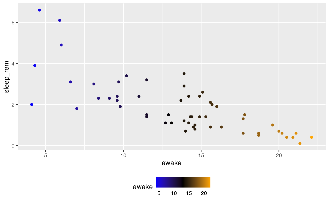

# Example of a fill gradient, still using points but with pch = 21, which accepts color and fill
ggplot(msleep_clean) + 
  aes(x = awake, 
      y = sleep_rem, 
      fill = awake) + # FILL is mapped to a continuous variable 
  geom_point(pch = 21,
             # Size is increased here just so you can better see the filled in points
             size = 2) +
  scale_fill_gradient(low = "blue", high = "orange")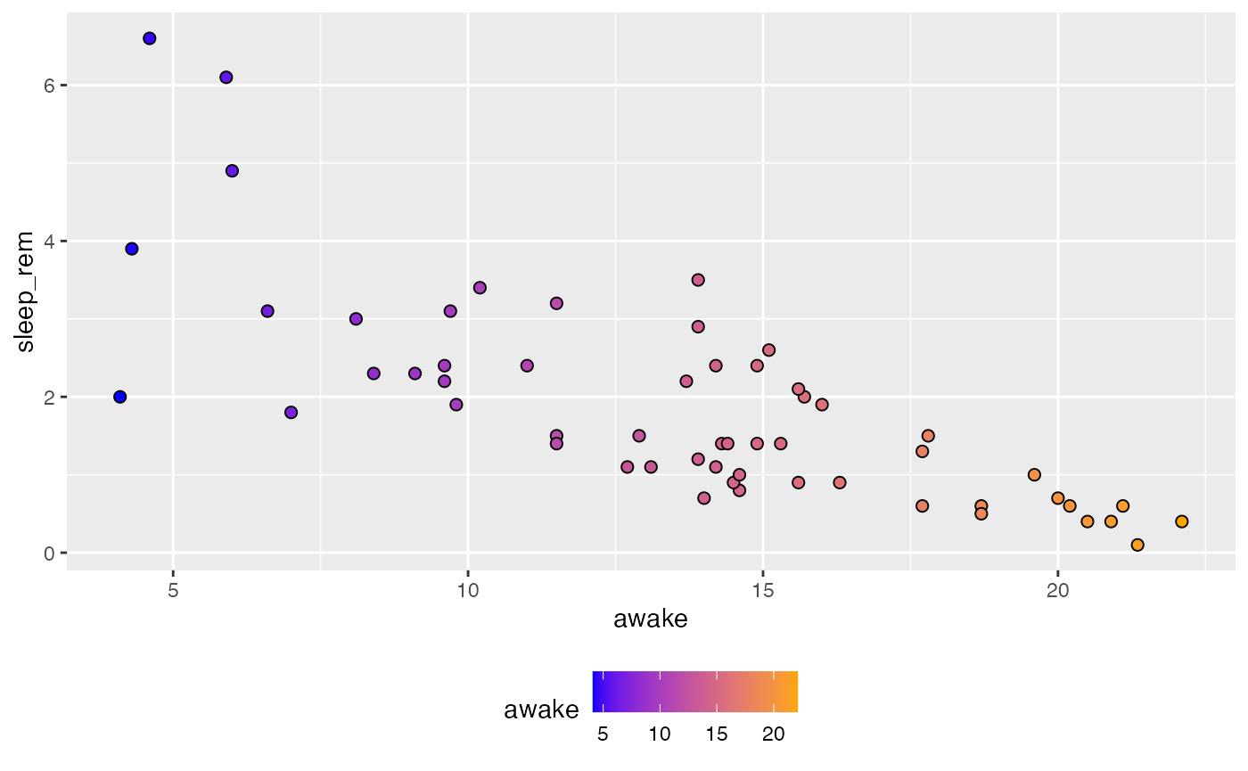

Using a colorbrewer scale

To use a colorbrewer palette with continuous data, use the function scale_<color/fill>_distiller() with the argument palette to specify which palette you want to use. Again, always make sure to use the right function name for the aesthetic you are considering. In other words, use scale_color_distiller() to customize a color mapping, not to customize a fill mapping.

# Specify custom _colors_ for each awake value
ggplot(msleep_clean) + 
  aes(x = awake, 
      y = sleep_rem, 
      color = awake) + 
  geom_point() +
  scale_color_distiller(palette = "Reds")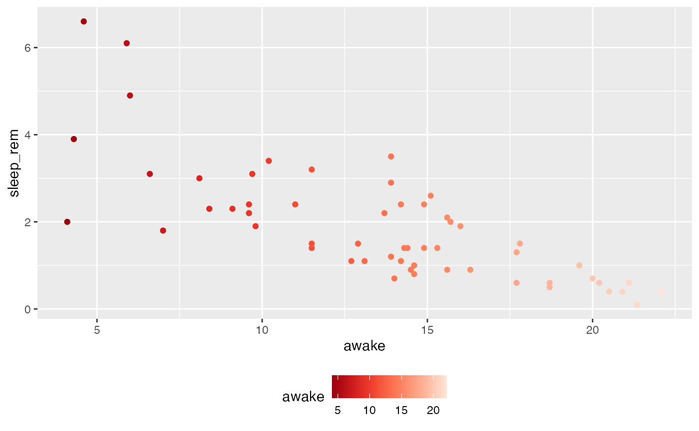

# Specify custom _fills_ for each awake value, still using points but with pch = 21, which accepts color and fill
ggplot(msleep_clean) + 
  aes(x = awake, 
      y = sleep_rem, 
      fill = awake) + 
  geom_point(pch = 21,
             # Size is increased here just so you can better see the filled in points
             size = 2) +
  # blue/purple distiller
  scale_fill_distiller(palette = "BuPu")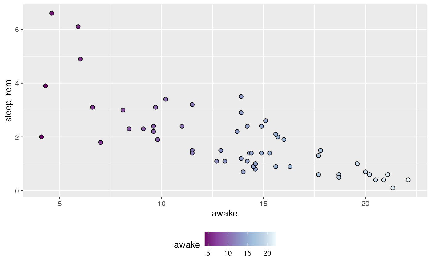

Using a viridis scale

To use a viridis palette with continuous data, use the function scale_<color/fill>_viridis_c() (c for continuous!) with the argument option (not palette) to specify which palette you want to use. Again, always make sure to use the right function name for the aesthetic you are considering. In other words, use scale_color_viridis_c() to customize a color mapping, not to customize a fill mapping.

# Specify custom _colors_ for each awake value
ggplot(msleep_clean) + 
  aes(x = awake, 
      y = sleep_rem, 
      color = awake) + 
  geom_point() +
  scale_color_viridis_c(option = "inferno")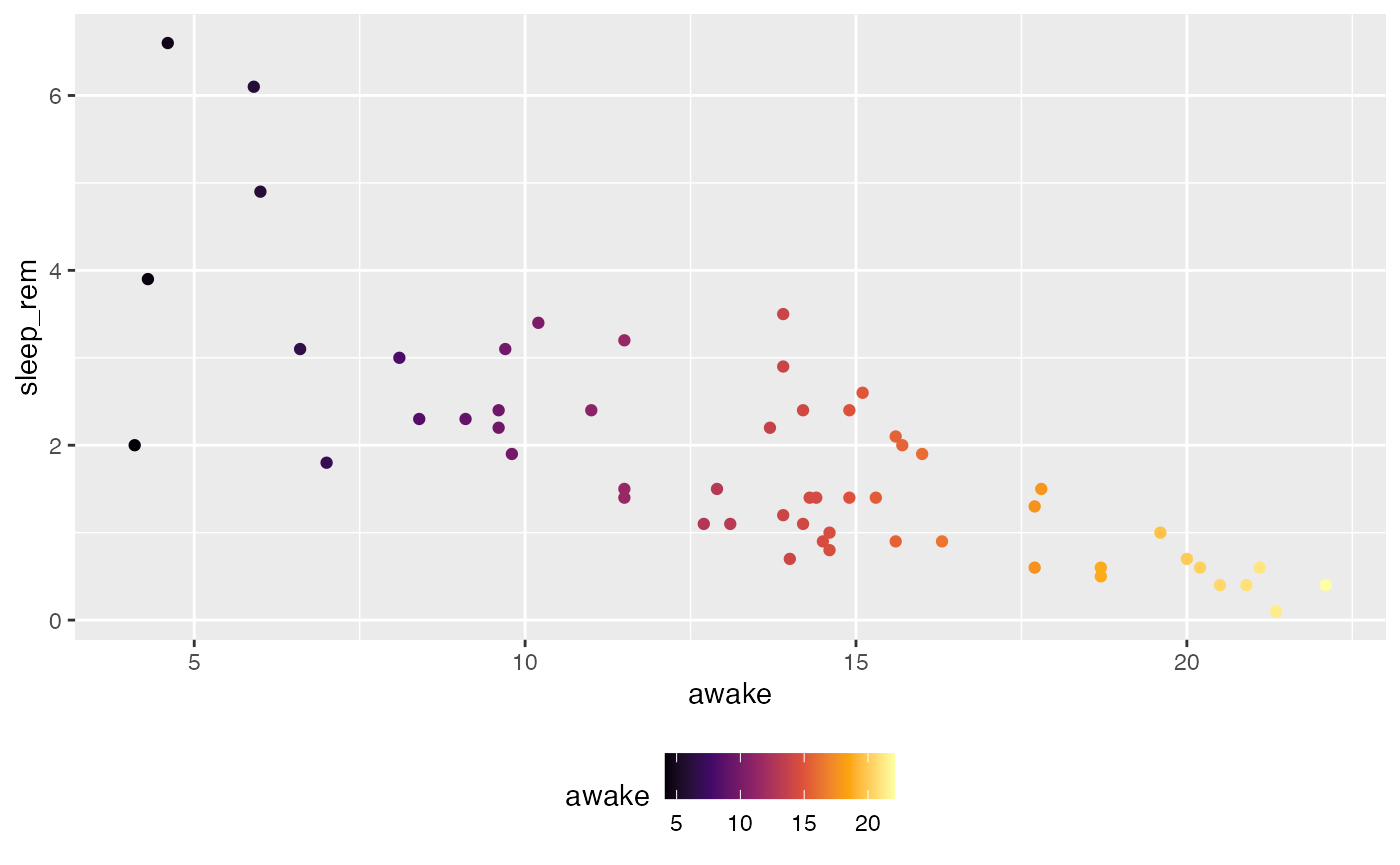

# Specify custom _colors_ for each awake value
ggplot(msleep_clean) + 
  aes(x = awake, 
      y = sleep_rem, 
      color = awake) + 
  geom_point() +
  # without `option`, the default viridis palette is used
  scale_color_viridis_c()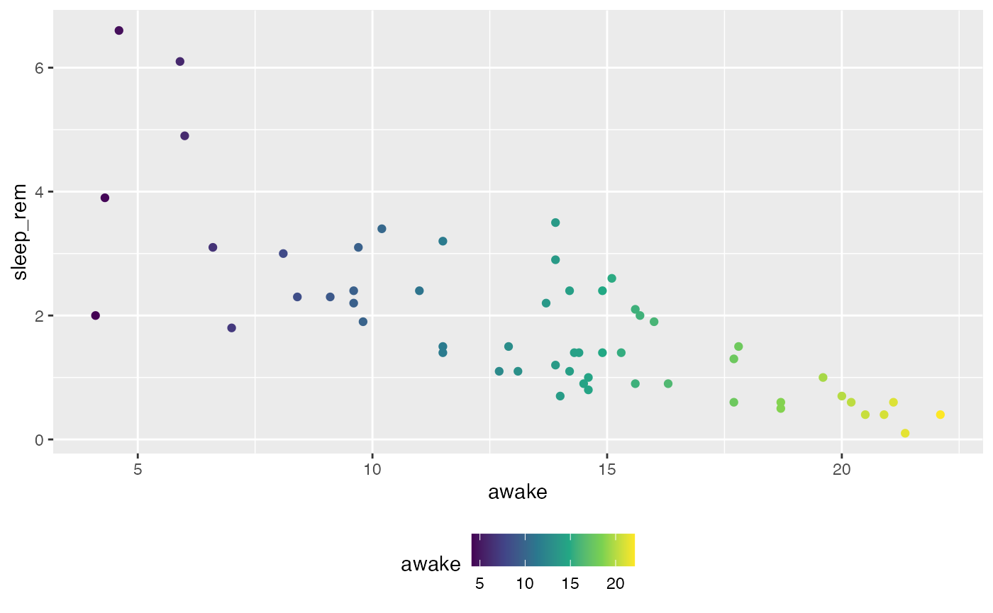

# You can reverse the order of the palette with `direction = -1`
# This argument works with any viridis function
ggplot(msleep_clean) + 
  aes(x = awake, 
      y = sleep_rem, 
      color = awake) + 
  geom_point() +
  # reverse the order of the palette
  scale_color_viridis_c(direction = -1)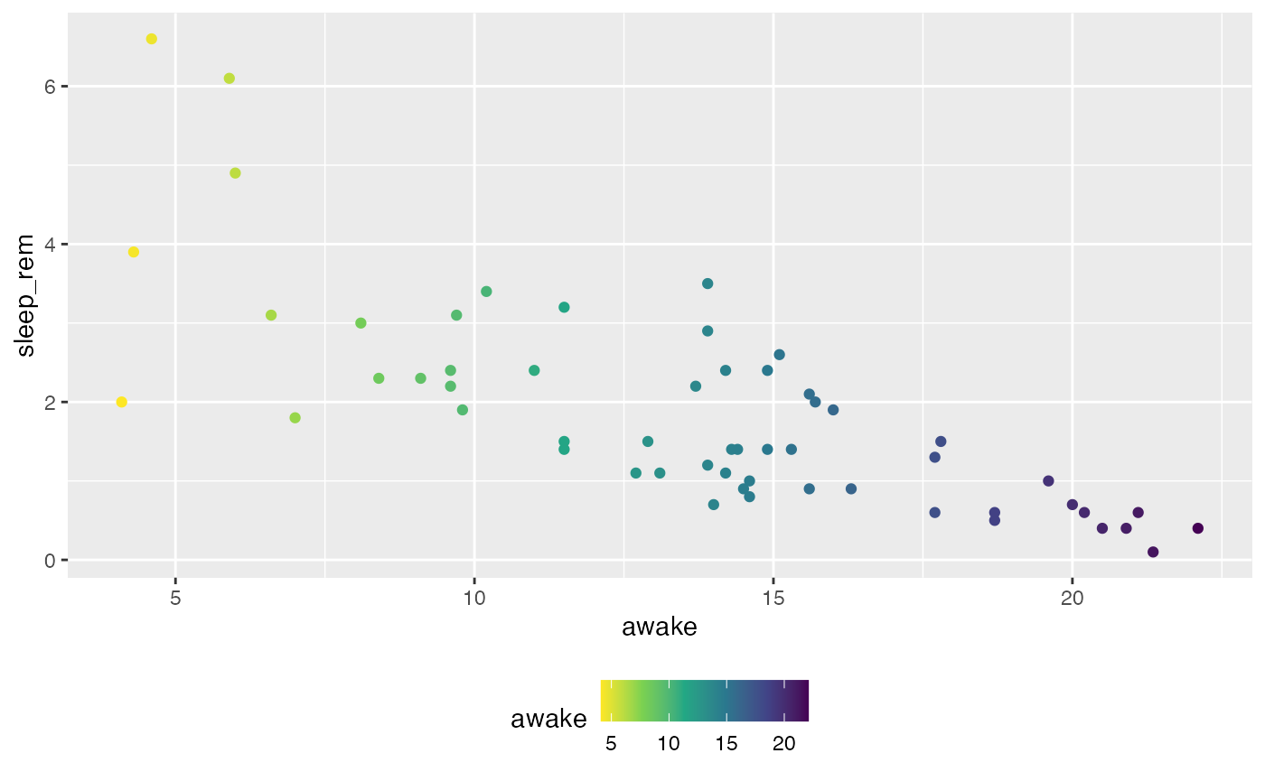

# Specify custom _fills_ for each awake value, still using points but with pch = 21, which accepts color and fill
ggplot(msleep_clean) + 
  aes(x = awake, 
      y = sleep_rem, 
      fill = awake) + 
  geom_point(pch = 21,
             # Size is increased here just so you can better see the filled in points
             size = 2) +
  scale_fill_viridis_c(option = "magma")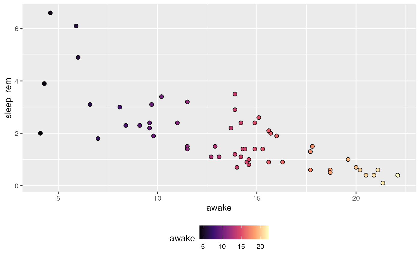

Dealing with NA values

In the previous examples, we removed all NA values from the columns we were plotting. However, if NA values are represent, they will be colored/filled gray (specifically, “gray50”) by default (with any palette). For example,

# Example scatterplot with NAs
ggplot(msleep_clean) + 
  aes(x = awake, 
      y = sleep_rem, 
      # Color points by sleep_cycle, a continuous variable with NA's 
      color = sleep_cycle) + 
  geom_point() -> na_scatterplot

# Example boxplot with NAs
ggplot(msleep_clean) + 
  aes(x = conservation, 
      y = awake, 
      # Fill by conservation, a discrete variable with NA's
      fill = conservation) + 
  geom_boxplot() -> na_boxplot

# Add plots together for display, which is allowed since `{patchwork}` has been loaded
na_scatterplot + na_boxplot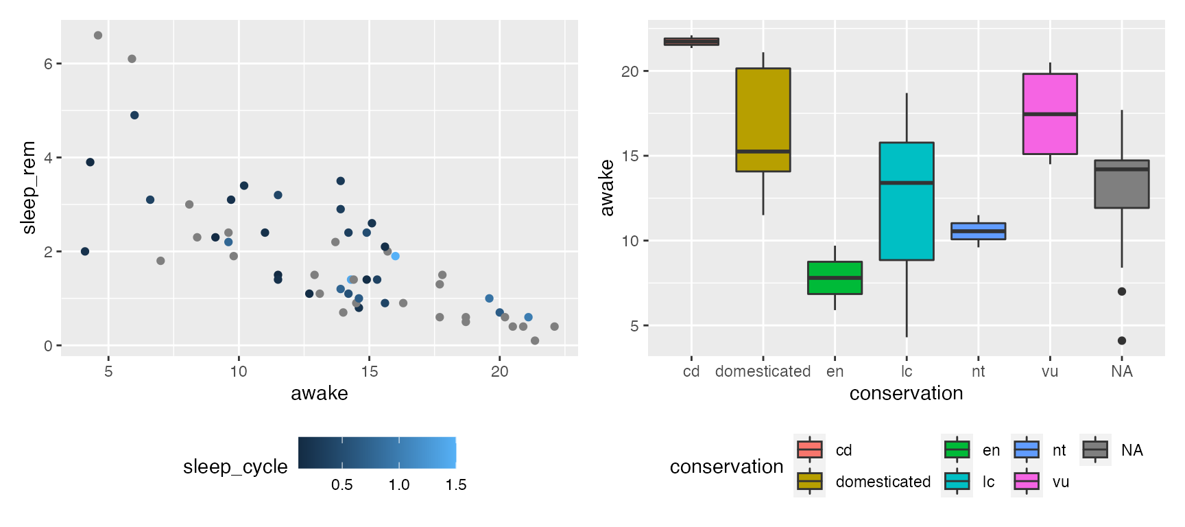

To override the default NA color or fill, provide a scale_ function with the argument na.value = COLOR YOU WANT NA's TO BE, as shown in examples below.

Using default {ggplot2} scales

If you want to change the NA color/fill while using the default ggplot2 scales, you will need to use one of these functions: + scale_<color/fill>_discrete() if the mapped variable is discrete/categorical + scale_<color/fill>_continuous() if the mapped variable is continuous

# Example scatterplot with NAs using default ggplot2 palette
# The discrete variable conservation is mapped to color, so use scale_color_discrete()
# We force NA colors to be yellow
ggplot(msleep) + 
  aes(x = awake, 
      y = sleep_rem, 
      # Color points by conservation, a discrete variable with NA's 
      color = conservation) + 
  geom_point() +
  scale_color_discrete(na.value = "yellow")
#> Warning: Removed 22 rows containing missing values (geom_point).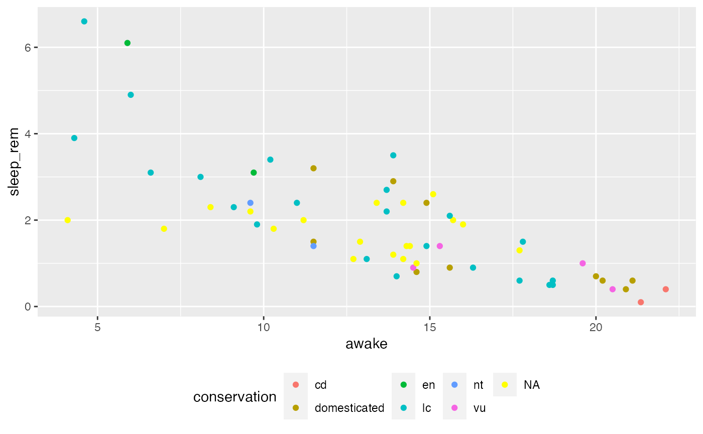

# Example scatterplot with NAs using default ggplot2 palette
# The continuous variable sleep_cycle is mapped to color, so use scale_color_continuous()
# We force NA colors to be yellow
ggplot(msleep) + 
  aes(x = awake, 
      y = sleep_rem, 
      # Color points by sleep_cycle, a continuous variable with NA's 
      color = sleep_cycle) + 
  geom_point() +
  scale_color_continuous(na.value = "yellow")
#> Warning: Removed 22 rows containing missing values (geom_point).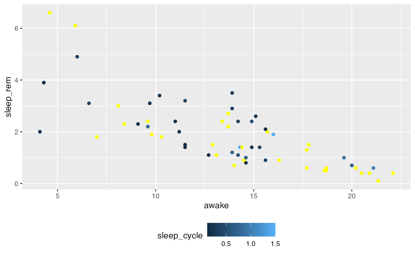

# Example boxplot with NAs using default ggplot2 palette
# The discrete variable conservation is mapped to fill, so use scale_fill_discrete()
# We force NA fills to be yellow
ggplot(msleep) + 
  aes(x = conservation, 
      y = awake, 
      # Fill points by conservation, a discrete variable with NA's 
      fill = conservation) + 
  geom_boxplot() +
  scale_fill_discrete(na.value = "yellow")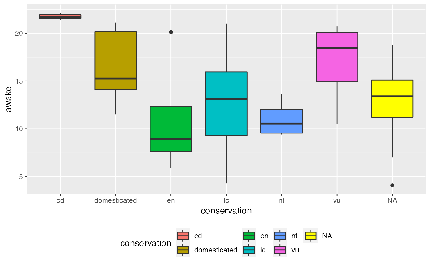

Using custom, colorbrewer, or viridis scales

Simply add in the argument na.value = COLOR FOR THE NA VALUES to any of the scale functions you have seen:

# Example scatterplot with NAs using a custom palette
# The continuous variable sleep_cycle is mapped to color, so use scale_color_gradient()
# We force NA colors to be yellow
ggplot(msleep) + 
  aes(x = awake, 
      y = sleep_rem, 
      # Color points by sleep_cycle, a continuous variable with NA's 
      color = sleep_cycle) + 
  geom_point() +
  scale_color_gradient(low = "orange", 
                       high = "brown", 
                       na.value = "yellow")
#> Warning: Removed 22 rows containing missing values (geom_point).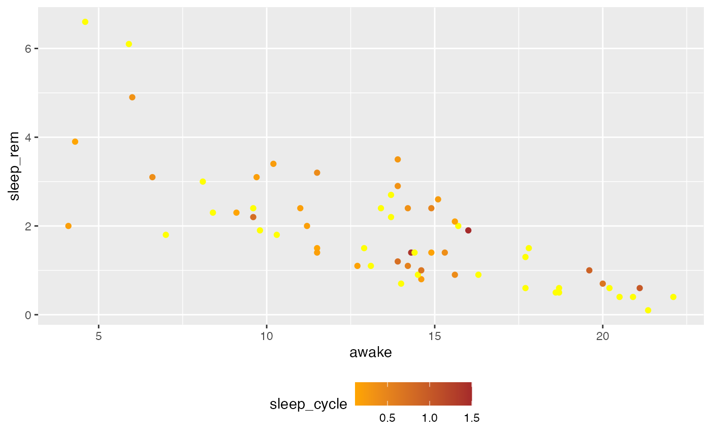

# Example scatterplot with NAs using a colorbrewer palette
# The continuous variable sleep_cycle is mapped to color, so use scale_color_distiller()
# We force NA colors to be yellow
ggplot(msleep) + 
  aes(x = awake, 
      y = sleep_rem, 
      # Color points by sleep_cycle, a continuous variable with NA's 
      color = sleep_cycle) + 
  geom_point() +
  scale_color_distiller(palette = "Purples",
                        na.value = "yellow")
#> Warning: Removed 22 rows containing missing values (geom_point).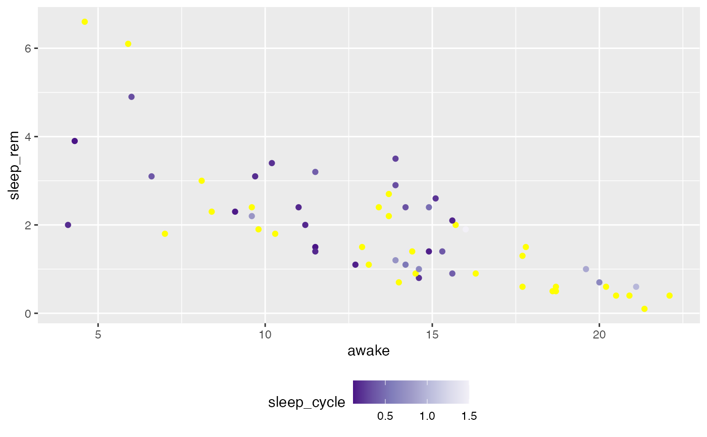

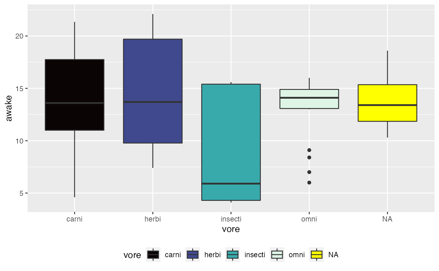
# Example boxplot with NAs using a viridis palette
# The discrete variable vore is mapped to fill, so use scale_fill_viridis_d()
# We force NA fills to be yellow
ggplot(msleep) + 
  aes(x = vore, 
      y = awake, 
      # Fill points by vore, a discrete variable with NA's 
      fill = vore) + 
  geom_boxplot() +
  scale_fill_viridis_d(option = "mako",
                       na.value = "yellow")