Introduction to Hypothesis Testing and Comparing Means

Lecture

Slides

R content

Sampling distribution of the mean

We consider here the population of platypus gene GC contents (full download available here). This population has a mean $\mu = 51.16$ and standard deviation $\sigma = 8.27$ :

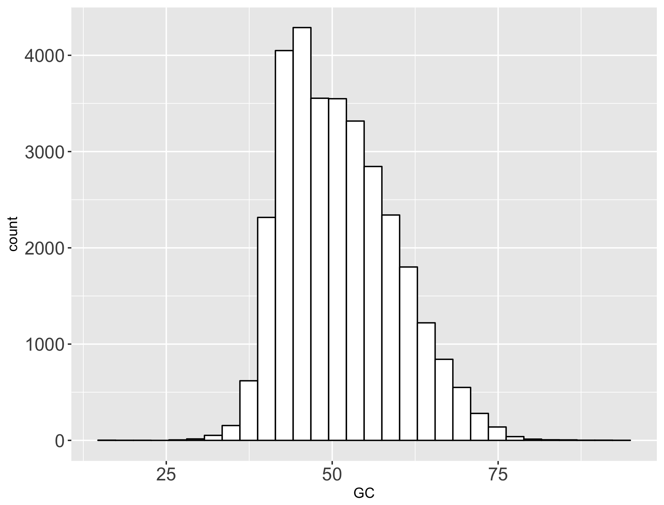
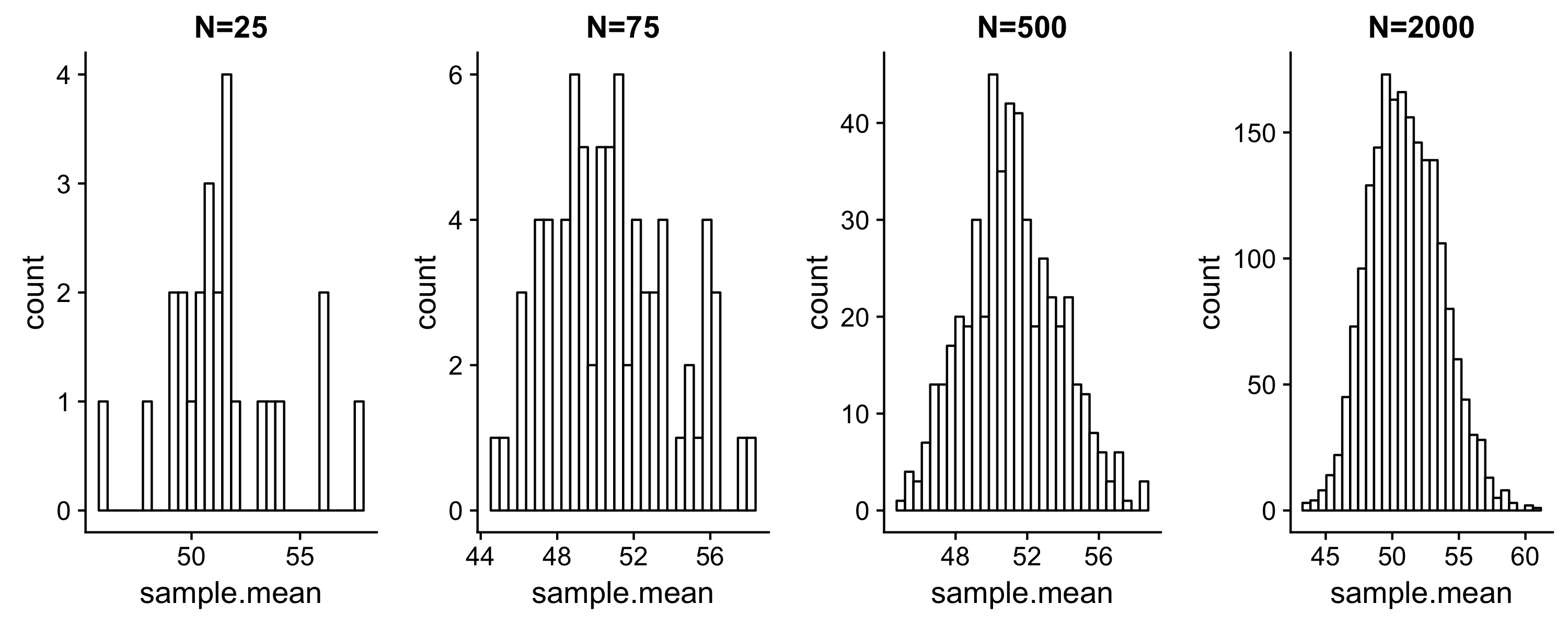
We will describe four sampling distributions of the mean from this population distribution. Each sampling distribution contains N sample means, computed from N random samples drawn from the population. You can download each here:



#### Read all datasets into R ####
n25 <- read_csv("platypus_gc_sampdist_n25.csv")
n75 <- read_csv("platypus_gc_sampdist_n75.csv")
n500 <- read_csv("platypus_gc_sampdist_n500.csv")
n2000 <- read_csv("platypus_gc_sampdist_n2000.csv")

#### Generate a histogram for each sampling distribution ####
ggplot(n25, aes(x = sample.mean)) + geom_histogram(fill = "white", color = "black") + ggtitle("N=25")
ggplot(n75, aes(x = sample.mean)) + geom_histogram(fill = "white", color = "black") + ggtitle("N=75")
ggplot(n500, aes(x = sample.mean)) + geom_histogram(fill = "white", color = "black")+ ggtitle("N=500")
ggplot(n2000, aes(x = sample.mean)) + geom_histogram(fill = "white", color = "black") + ggtitle("N=2000")



#### Compute SE for N=<25,75,500,2000> sampling distributions of the mean
se.n25_true <- 8.27/sqrt(25)
se.n75_true <- 8.27/sqrt(75)
se.n500_true <- 8.27/sqrt(500)
se.n2000_true <- 8.27/sqrt(2000)


#### Compute mean and SE for each. ####
mean.n25 <- mean(n25$sample.mean)
se.n25_sample  <- sd(n25$sample.mean)/sqrt(25)

mean.n75 <- mean(n75$sample.mean)
se.n75_sample <- sd(n75$sample.mean)/sqrt(75)

mean.n500 <- mean(n500$sample.mean)
se.n500_sample <- sd(n500$sample.mean)/sqrt(500)


mean.n2000 <- mean(n2000$sample.mean)
se.n2000_sample <- sd(n2000$sample.mean)/sqrt(2000)

Values computed in code above are seen in tables:

Parameter SE:

N	SE
25	1.654
75	0.955
500	0.34
2000	0.18

Sample estimates

N	Mean	Sample SE
25	51.4	0.53
75	50.99	0.36
500	51.17	0.16
2000	51.02	0.06

To compute the standard error of the sampling distribution of the means, we using the population standard deviation $\sigma$ (“Parameter SE” table). This is the standard deviation of the sampling distribution of the mean for N=n.

$\sigma_\bar{x} = \sigma / \sqrt{n}$

In the case where we do not know the population parameters and we are estimating from a sample, we must compute the standard error approximately using the sample standard deviation $s$ (“Sample estimates” in table):

$SE_\bar{x} = s / \sqrt{n}$

As N increases, we expect the following:
- The mean of the sampling distribution should approach the population mean
- The standard error should decrease, indicating that we are reaching the mean with increasing precision

Performing t-tests in R

The following examples all utilize the same data set, for explanatory purposes. In general, do not perform multiple tests on the same data, until we have learned how to do so safely later this semester.

Setting up your t-test

Use the function t.test() as follows:

One-sample, two-tailed: t.test(<vector of data>, mu = <null value>)
One-sample, one-tailed:
- Test $x > \mu$ : t.test(<vector of data>, mu = <null value>, alternative = "greater")
- Test $x < \mu$ : t.test(<vector of data>, mu = <null value>, alternative = "less")
Two-sample, two-tailed: t.test(<first vector of data>, <second vector of data>)
Two-sample, one-tailed:
- Note the order of vectors provided - first argument is considered $\mu_1$ .
- Test $\mu_1 > \mu_2$ : t.test(<first vector of data>, <second vector of data>, alternative = greater).
- Test $\mu_1 < \mu_2$ : t.test(<first vector of data>, <second vector of data>, alternative = "less")
Paired t-test can be run in two ways:
- Like one-sample tests with the <vector of data> containing the difference between samples and null of mu=0
- Like two-sample tests with the added argument paired=TRUE

One-sample t-tests: Two-sided

We will test the following hypothesis using $\alpha = 0.05$ :

Ho: The mean of virginica iris Sepal Lengths equals 6.15
Ha: The mean of virginica iris Sepal Lengths does not equal 6.15

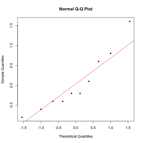
First, check that the data is normally distributed:



### Subset data
> virginica <- iris %>% filter(Species == "virginica")

### Generate normal Q-Q plot
> qqnorm(virginica$Sepal.Length, pch=20)
> qqline(virginica$Sepal.Length, col="red")

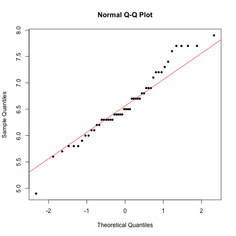
Data follow the Q-Q line. Therefore data are normally distributed and we can perform the test:



> t.test(virginica$Sepal.Length, mu = 6.15)
			One Sample t-test
		
		data:  virginica$Sepal.Length
		t = 4.8706, df = 49, p-value = 1.204e-05
		alternative hypothesis: true mean is not equal to 6.15
		95 percent confidence interval:
		 6.407285 6.768715
		sample estimates:
		mean of x 
		    6.588

Our test statistic is 4.87 with 49 degrees of freedom. The P-value is $1.2\times10{-5}$ , which is less than our $\alpha$ of 0.05. We therefore reject the null hypothesis and conclude that there is evidence that virginica sepal lengths differ from 6.15. We can further conclude that virginica sepal lengths are larger than 6.15 (sample mean = 6.59). We have a 95% confidence interval of [6.41, 6.76], meaning there is a 95% chance that the true population mean falls in this range. Indeed, the null of 6.15 does not fall in this interval, reflecting our significant result.

One-sample t-tests: One-sided

We will test the following hypothesis using $\alpha = 0.05$ :

Ho: The mean of virginica iris Sepal Lengths equals 6.15
Ha: The mean of virginica iris Sepal Lengths is greater than 6.15

We have already confirmed assumptions above. Therefore proceed to test:



## Specify alternative = "greater" to obtain P-value from upper tail only, consistent with provided hypothesis
> t.test(virginica$Sepal.Length, mu = 6.15, alternative = "greater")
			One Sample t-test
		
		data:  virginica$Sepal.Length
		t = 4.8706, df = 49, p-value = 6.02e-06
		alternative hypothesis: true mean is greater than 6.15
		95 percent confidence interval:
		 6.437233      Inf
		sample estimates:
		mean of x 
		    6.588

Most reslts are the same as before with a few differences:

The P-value is $6.02\times10{-6}$ . As expected, this is half the value of our two-sided t-test
The CI has an upper bound of infinity, because we performed a one-sided test. This is expected.

We will test the following hypothesis using $\alpha = 0.05$ :

Ho: The mean of virginica iris Sepal Lengths equals 6.15
Ha: The mean of virginica iris Sepal Lengths is less than 6.15

We have already confirmed assumptions above. Therefore proceed to test:



## Specify alternative = "less" to obtain P-value from lower tail only, consistent with provided hypothesis
> t.test(virginica$Sepal.Length, mu = 6.15, alternative = "less")
			One Sample t-test
		
		data:  virginica$Sepal.Length
		t = 4.8706, df = 49, p-value = 1
		alternative hypothesis: true mean is less than 6.15
		95 percent confidence interval:
		     -Inf 6.738767
		sample estimates:
		mean of x 
		    6.588

Here, we have a P-value of 1, which a is a result of rounding $1 - 6.02\times10{-6} = 0.999994 \approx 1$ . Whenever we have a P-value > 0.5, we have made the wrong directional choice. With P-value = 1, we fail to reject the null hypothesis. We have no evidence that virginica sepal lengths are shorter than 6.15. Our conclusion is further reflected in the CI, because the null 6.15 is is the interval.

Two-sample t-tests: One-sided

We will test the following hypothesis using $\alpha = 0.05$ :

Ho: The mean of virginica iris Sepal Lengths equals the mean of versicolor iris Sepal Lengths
Ha: The mean of virginica iris Sepal Lengths is greater than the mean of versicolor iris Sepal Lengths.

First, check that the data is normally distributed. Since we checked above already for viriginica, we will check now for versicolor only.



### Subset data
> versicolor <- iris %>% filter(Species == "versicolor")

### Generate normal Q-Q plot
> qqnorm(versicolor $Sepal.Length, pch=20)
> qqline(versicolor $Sepal.Length, col="red")

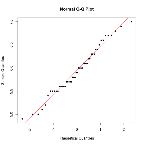
We now have confirmed that both samples are normal, so proceed to test.



## Specify alternative = "less" to obtain P-value from lower tail only, consistent with provided hypothesis, making sure to provide virginica first!
> t.test(virginica$Sepal.Length, versicolor$Sepal.Length, alternative = "greater")

			Welch Two Sample t-test
		
		data:  virginica$Sepal.Length and versicolor$Sepal.Length
		t = 5.6292, df = 94.025, p-value = 9.331e-08
		alternative hypothesis: true difference in means is greater than 0
		95 percent confidence interval:
		 0.4595885       Inf
		sample estimates:
		mean of x mean of y 
		    6.588     5.936 
## Compute effect size
> 6.588 - 5.936	   
   [1] 0.652

Our test statistic is 5.6292 with 94.025 degrees of freedom. The P-value is $9.3\times10{-8}$ , which is less than our $\alpha$ of 0.05. We therefore reject the null hypothesis and conclude that there is evidence that virginica sepal lengths are larger than versicolor sepal lengths. The effect size is 0.652, meaning on average virginica sepal lengths are 0.652 cm longer than versicolor. We have a 95% confidence interval of [0.46, Inf], meaning there is a 95% chance that the true difference in means falls in this range. Our conclusion is further reflected in the CI, because 0 (the null difference between means) is not in this CI.

Two-sample t-tests: Two-sided

We will test the following hypothesis using $\alpha = 0.05$ :

Ho: The mean of virginica iris Sepal Lengths equals the mean of versicolor iris Sepal Lengths
Ha: The mean of virginica iris Sepal Lengths does not equal the mean of versicolor iris Sepal Lengths.

We already confirmed assumptions above, so we can proceed to the test.



> t.test(virginica$Sepal.Length, versicolor$Sepal.Length)
			Welch Two Sample t-test
		
		data:  virginica$Sepal.Length and versicolor$Sepal.Length
		t = 5.6292, df = 94.025, p-value = 1.866e-07
		alternative hypothesis: true difference in means is not equal to 0
		95 percent confidence interval:
		 0.4220269 0.8819731
		sample estimates:
		mean of x mean of y 
		    6.588     5.936 

## Compute effect size
> 6.588 - 5.936	   
   [1] 0.652

Our test statistic is 5.6292 with 94.025 degrees of freedom. The P-value is $1.87\times10{-8}$ , which is twice the value of our analogous one-sided P-value. It is also less than our $\alpha$ of 0.05. We therefore reject the null hypothesis and conclude that there is evidence that virginica sepal lengths differ from versicolor sepal lengths. Because of our significant result, we can make a directional conclusion (even though we did not perform a directional test): virginica are longer than versicolor, based on effect size of 0.652. We have a 95% confidence interval of [0.42, 0.88], meaning there is a 95% chance that the true difference in means falls in this range. Our conclusion is further reflected in the CI, because 0 (the null difference between means) is not in this CI.

Paired t-tests: Two-sided

This example uses this example scenario: The 100-meter running time for 10 athletes is recorded before and after training (ordered by individual):

Before training: 12.9, 13.5, 12.8, 15.6, 17.2, 19.2, 12.6, 15.3, 14.4, 11.3 After training: 12.7, 13.6, 12.0, 15.2, 16.8, 20.0, 12.0, 15.9, 16.0, 11.1

We will test the following: Ho: Athletes running time is the same before and after training. Ha: Athletes running time differs before and after training.

First, check the assumption that the difference between data points is normal:


## Make the dataset:
atheletes <- tibble(before = c(12.9, 13.5, 12.8, 15.6, 17.2, 19.2, 12.6, 15.3, 14.4, 11.3), after = c(12.7, 13.6, 12.0, 15.2, 16.8, 20.0, 12.0, 15.9, 16.0, 11.1))

## Check the difference for normality
atheletes <- atheletes %>% mutate(diff = after - before)
qqnorm(atheletes$diff, pch=20)
qqline(atheletes$diff, col="red")

The assumption is met, so proceed to test:


## Code version one: Run as one-sample with mu = 0 
> t.test(atheletes$diff, mu = 0)
			One Sample t-test
		
		data:  atheletes$diff
		t = 0.21331, df = 9, p-value = 0.8358
		alternative hypothesis: true mean is not equal to 0
		95 percent confidence interval:
		 -0.4802549  0.5802549
		sample estimates:
		mean of x 
		     0.05 
		     
> t.test(atheletes$after, atheletes$before, paired=T)
			Paired t-test
		
		data:  atheletes$after and atheletes$before
		t = 0.21331, df = 9, p-value = 0.8358
		alternative hypothesis: true difference in means is not equal to 0
		95 percent confidence interval:
		 -0.4802549  0.5802549
		sample estimates:
		mean of the differences 
		                   0.05

Our test statistic is 0.21331 with 9 degrees of freedom. The P-value is 0.84, which is greater than our $\alpha$ of 0.05. We therefore fail to reject the null hypothesis and conclude that there is no evidence in this data that training affected 100-meter runtime.