Introduction to R and RStudio

Other resources

Here are some other great resources for introducing R, but please be aware that not all of the content introduced below will be specifically relevant to our class. It is definitely all relevant to fully mastering R, however.

Why use R?
More! Why use R?
R Basics from the STAT545 course by Jenny Bryan at UBC
Introduction to R from Data Carpentry
Starting out with R
R Tutorial

What is R?

R is a statistical computing language that is open source, meaning the underlying code for the language is freely available to anyone. You do not need a special license or set of permissions to use and develop code in R.

R itself is an interpreted computer language¹. We use the term “base R” to refer to R’s functionality that comes bundled with the language itself. There is rich additional functionality provided by external packages, or libraries of code that assist in accomplishing certain tasks. These packages, also referred to as libraries, can be freely downloaded and loaded for use. This class will be focused on learning how to use some really important data science packages, including ggplot2 for data visualization and dplyr for data manipulation and “wrangling.” We will not focus on using base R.

What is RStudio?

RStudio is a graphical environment (“integrated development environment” or IDE) for writing and developing R code. RStudio is NOT a programming language - it is an interface (“app”) we use to facilitate R programming. In other words, you can program in R without RStudio, but you can’t use the RStudio environment without R²

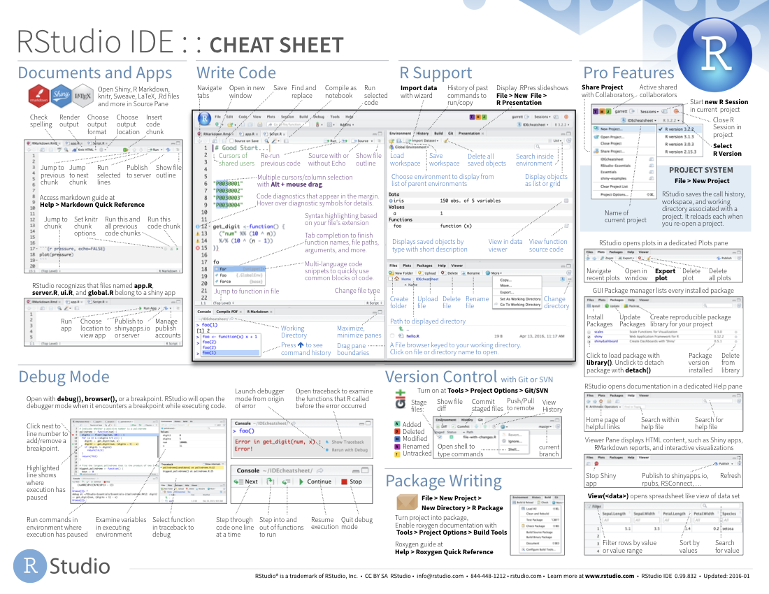
For more information about RStudio than you ever wanted to know, see this RStudio IDE Cheatsheet.

Obtaining and Using R/RStudio

There are two main paths to developing in R within the RStudio environment:

Use RStudio in the browser via rstudio.cloud. Make your free account on this website and you can get started right away. For this class, we will be using RStudio Cloud! This option requires NO downloads at all.
Download and install both R and RStudio (in that order!) to your local machine. This requires some amount of computer knowledge, and not all computer operating system versions will be compatible. If you anticipate serious R usage in your future, you will eventually want to do this.
- Link to download R
- Link to download RStudio (click the free version!)

The RStudio Environment

The RStudio environment has four main panes (their specific location can be changed under Tools -> Global Options -> Pane Layout). RStudio Appearance

This image presents the RStudio Cloud environment within a project I have created called “demo” and an R script called “example.R”. Note that this screenshot was taken when the R language was at verion 3.6.0. As of January 2021, the language is now at version 4.0.3, but for our purposes this distinction doesn’t matter at all.

The editor pane is where you can write R scripts and other documents. This is your text editor, which will allow you to save your R code for future use. R scripts can also directly be run from this pane. In this image, you can see an R script called “example.R” which contains some simple R to define and print a variable. But be aware, when there is no file open, this pane will automatically collapse and disappear from view. You can always open it again by opening a file.
The console pane is where you can interactively run R code. You can also use this pane as a terminal to emulate a UNIX shell (please ignore this if you are unfamiliar with UNIX). In this image, you can see that the user has defined a variable called “y” and printed out its value. In the console, new lines where you can type code are indicated by greater than signs > - we do not type these symbols - R places them there to indicate a new line is starting.
The environment pane primarily displays the variables, sometimes known as objects you define during a given R session. You can ignore its other tabs for now. In this image, you can see that a variable “y” has been created with the value “9” (see the “console” code?). You’ll also notice that the variable “x” is not listed in the environment pane - that’s because the script “example.R” has only been written but not (yet!) run, so R doesn’t know about it.
The files, plots, packages, help, viewer pane has several tabs all of which are pretty important:
- The files tab shows the structure and contents of your current directory (i.e. folder). In the example image, the user is working in a directory (folder!) called “project”, and this directory contains THREE files: .Rhistory, project.Rproj, and example.R - the file shown in the editor pane. For now, don’t worry about what the first two files are.
- The plots tab will reveal plots when you make them
- The packages tab shows which installed packages have been loaded into your R session
- The help tab will show the help page when you look up a function
- The viewer pane will reveal compiled RMarkdown documents (stay tuned 2 more weeks)

You can change your preferred panel organization by clicking on the grid icon, which reveals a dropdown menu for moving panes to your preferred side (left/right) or layer (top/bottom).

Comments

Arguably the most important aspect of your coding is comments: Small pieces of explanatory text you leave in your code to explain what the code is doing and/or leave notes to yourself or others. Comments are invaluable for communicating your code to others, but they are most important for Future You. Future You comes into existence about one second after you write code, and has no idea what on earth Past You was thinking. Help out Future You by adding lots of comments! Future You next week thinks Today You is an idiot, and the only way you can convince Future You that Today You is reasonably competent is by adding comments in your code explaining why Today You is actually not so bad.

R will ignore comments, which are indicated with hashtags. Anything on a given line that appears after a hashtag will be ignored, whether the hashtag is at the beginning of a line or in the middle of a line. You will see many comments in example code below!

R as a calculator

The most basic use of R is as a regular calculator:

Operation	Symbol
Add	`+`
Subtract	`-`
Multiply	`*`
Divide	`/`
Exponentiate	`^` or `**`

For example, we can do some simple multiplication like this. In this and following code chunks, the section with the gray background is R code, and the following white-background chunk is the code’s output.

12 * 10
## [1] 120

Working with variables

Defining variables

To define a variable, we use the assignment operator which looks like an arrow: <-. It is a less than sign immediately followed by a minus sign - no spaces!!!

For example x <- 7 takes the VALUE on the right-hand side of the operator and ASSIGNS it to the VARIABLE NAME on the left-hand side. The opposite is also possible, e.g. 7 -> x (minus sign THEN a greater than sign - an arrow pointing the other way.

As long as the arrow is pointing FROM the value and towards the VARIABLE NAME, you are good:

# Define a variable x to equal 7, and print out the value of x
x <- 7
x
## [1] 7
# This also works. Always point FROM the value, TO the variable.
7 -> x
x
## [1] 7

Pointing the other direction leads to errors. 7 is 7 is 7 - you can’t make 7 into x:

# Not allowed
x -> 7
## Error in 7 <- x: invalid (do_set) left-hand side to assignment
# Similarly, not allowed
7 <- x
## Error in 7 <- x: invalid (do_set) left-hand side to assignment

Some features of variables, considering the example x <- 7:

Every variable has a name, a value, and a type. This variable’s name is x, its value is 7, and its type is numeric (7 is a number!). We will learn more about variable types soon.
Variable names can be any string, i.e. a set of characters (numbers, letters, and cerain symbols). Variables names should start with a letter, and it is best practice to avoid all symbols EXCEPT underscores. Never use periods, dollar signs, or spaces. If you do, you will learn this the hard way.
Variable names are case sensitive, meaning it matters if you use upper or lower case letters. If we try to access the variable X (capitalized), we will get an error because it is undefined:
```
print(x) # works!
## [1] 7
print(X) # error :(
## Error in print(X): object 'X' not found
```
Re-defining a variable will OVERWRITE the value.
```
x
## [1] 7
x <- 5.5

x
## [1] 5.5
```
As best you can, it is a good idea to make your variable names informative (e.g. x doesn’t mean anything, but cost_of_sandwich is meaningful… if we’re talking about sandwich prices, that is..). Similarly, it is best practice to use underscores _ to separate words if there are multiple words in the name.

Variable Types

The example above defines a numeric variable - a variable whose value is a number. There are several other data types that values can have. Here are some of the most important types we’ll need to know:

Variable Type	Definition	Examples	Coersion
`numeric`	Any number value	`5` `7.5` `-1` `pi` (This is a constant variable defined in R as 3.1415…)	`as.numeric()`
`character`	Any collection of characters defined within quotation marks. Also known as a “string”.	`"a"` (a single letter) `"stringofletters"` (a whole bunch of characters put together as one) `"string of letters and spaces"` `"5"` `'single quotes are also good'`	`as.character()`
`logical`	A value of `TRUE`, `FALSE`, or `NA`	`TRUE` `FALSE` `NA` (not defined)	`as.logical()`
`factor`	A special type of data in R that denotes specific CATEGORIES of a categorical variable	(stay tuned..)	`as.factor()`

Variable types in R are what is known as “weakly typed”, meaning when possible, you can coerce (convert) one type to another.

For example, we can coerce an numeric to be a character:

x_numeric <- 15
class(x_numeric)
## [1] "numeric"
x_character <- as.character(x_numeric)
# See it now has quotes around it? It's now a character and will behave as such
x_character
## [1] "15"
class(x_character)
## [1] "character"
# aka, we can't add characters! even though "15" looks like a number, it's not
x_numeric + 4 # yay!
## [1] 19
x_character + 4 # nope
## Error in x_character + 4: non-numeric argument to binary operator

But we can’t coerce characters to be numerics:

# Define an integer
my_string <- "look at my character variable"
class(my_string)
## [1] "character"
# failed coersion. there is no natural way for a sentence to be numbers
# R decided the it's numeric version is undefined: NA
as.numeric(my_string)
## Warning: NAs introduced by coercion
## [1] NA

Logical variables and operators

One of the most important variable types are logical variables (known as “boolean” in many other languages). They help us to compare different quantities and there is a special set of operators for performing comparisons that return logical values:

Operator	What it does
`==`	Tests if two quantities are EQUAL. DOUBLE EQUALS SIGN IS SO IMPORTANT. DOUBLE. ~NOT SINGLE~
`>` and `<`	Tests if one quantity is greater than or less than another
`>=` and `<=`	Tests if one quantity is greater than or equal to or less than or equal to another
`!`	Negates an operation

Let’s examine their usage:

5 == 5
## [1] TRUE
7 >= 9
## [1] FALSE
4 < 8
## [1] TRUE
!(4 > 8)  # 4 is not greater than 8. Inside parentheses is FALSE, but the `!` negates the FALSE --> TRUE
## [1] TRUE
# Your most common mistake: Using a single equals sign to compare values.
# R says you can't define a variable called 4 and make it equal 3. 4 is already a thing. It's 4.
4 = 3
## Error in 4 = 3: invalid (do_set) left-hand side to assignment

Multiple logical operations

Logical conditions can also be combined with one another to make more involved True/False comparisons. For example, what if we want all values X where 5 < X < 20? This will require a more complex logical expression and the knowledge of two primary concepts:

and is True when BOTH conditions are True. (represented in R with the symbol &)
or is True when AT LEAST ONE condition is True (represented in R with the symbol | located on the backslash key! This is not the letter L or number 1; it is a “pipe” operator.)

For example:

############# and #################
10 > 5 & 5 == 5 ## Both are TRUE. 
## [1] TRUE
10 < 5 & 5 < 2 ## Both are FALSE.
## [1] FALSE
10 < 5 & 5 > 2 ## First is FALSE, second is TRUE.
## [1] FALSE
# Remember, use a _leading_ ! to negate
10 > 5 & !(5 < 2) ## Both are TRUE. 
## [1] TRUE
############ or ##############
10 == 10 | 10 == 11  ## First is TRUE, second is FALSE.
## [1] TRUE
10 == 10 | !(10 == 11) ## First is TRUE, second is TRUE.
## [1] TRUE
10 < 4 | 10 == 11  ## First is FALSE, second is FALSE. 
## [1] FALSE
########### get crazy with it ###########
!(10 < 4 & 77 == 33)   # Within parentheses evaluates to FALSE, but the external ! changes things..
## [1] TRUE

Functions

We can use pre-built computation methods called “functions” for other operations. In fact, we’ve already seen and used one - the print() function.

Functions have the following format, where the argument is the information we are providing to the function for it to run.

function_name(argument)

# Sometimes there are multiple arguments
function_name(argument1, argument2, argument3)

To learn about functions, we’ll examine one called log() first.

To know what a function does and how to use it, use the question mark which will reveal documentation in the help pane: ?log rhelp

The documentation tells use that log() is derived from {base}, meaning it is a function that is part of base R. It provides a brief description of what the function does and shows several examples of to how use it.

In particular, documentation tells about how what argument(s) to provide:]

The first required argument is the value we’d like to take the log of, by default its natural log
The second optional argument can specify a different base rather than the default e:

# Natural log of 2:
log(2)
## [1] 0.6931472
# Log of 2 in base 10:
log(2, 10)
## [1] 0.30103

Functions also return values for us to use. In the case of log(), the returned value is the log’d value the function computed.

One way you can tell the difference between variables and functions is that functions always have PARENTHESES, but variables do not!!

Arrays/vectors

You will have noticed that all your computations tend to pop up with a [1] preceding them in R’s output. This is because, in fact, all (ok mostly all) variables are by default arrays aka vectors, and our answers are the first (in these cases only) value in the array. As arrays gets longer, new index indicators will appear at the start of new lines. See here for a deeper dive into array structures.

# This is actually an array that has one item in it.
x <- 7

# The length() functions tells us how long an array is:
length(x)
## [1] 1
# In fact, a single STRING has a length of ONE!! Compare the new function `length()` to `nchar()`
name <- "Stephanie"
nchar(name)
## [1] 9
length(name)
## [1] 1

We can define arrays with the function c(), which stands for “combine”. This function takes a comma-separated set of values to place in the array, and returns the array itself:

my_numeric_array <- c(1,1,2,3,5,8,13,21)
my_numeric_array
## [1]  1  1  2  3  5  8 13 21
length(my_numeric_array)
## [1] 8
# Combining two arrays will make one BIGGER array, not a nested array
my_array_of_arrays <- c(my_numeric_array,  c(100,101,102))
my_array_of_arrays
##  [1]   1   1   2   3   5   8  13  21 100 101 102
length(my_array_of_arrays)
## [1] 11
# We can build on arrays in place by redefining them
my_numeric_array <- c(my_numeric_array, 10000)
my_numeric_array
## [1]     1     1     2     3     5     8    13    21 10000

If you want to quickly make an array of whole numbers in ascending order, you can also use a colon as low:high:

values_1_to_20 <- 1:20
values_1_to_20
##  [1]  1  2  3  4  5  6  7  8  9 10 11 12 13 14 15 16 17 18 19 20

One major benefit of arrays is the concept of vectorization, where R by default performs operations on the entire array at once. For example, we can get the log of all numbers 1-2 with a single, simple call, and more!

log(values_1_to_20)
##  [1] 0.0000000 0.6931472 1.0986123 1.3862944 1.6094379 1.7917595 1.9459101
##  [8] 2.0794415 2.1972246 2.3025851 2.3978953 2.4849066 2.5649494 2.6390573
## [15] 2.7080502 2.7725887 2.8332133 2.8903718 2.9444390 2.9957323
# Multiple all items by 10
10 * values_1_to_20
##  [1]  10  20  30  40  50  60  70  80  90 100 110 120 130 140 150 160 170 180 190
## [20] 200

Finally, we can apply logical expressions to arrays, just we can do for single values.

# Define an array of values ranging from 2-8
example_array <- 2:8 
example_array
## [1] 2 3 4 5 6 7 8
# Which values are <= 3?
# The output here is a LOGICAL ARRAY telling us whether each value in example_array is TRUE or FALSE
example_array <= 3
## [1]  TRUE  TRUE FALSE FALSE FALSE FALSE FALSE

A note on protected variables

A key concept that emerges here is protected variables. We have learned functions such as c(), length(), log(), etc. and more. Many computer languages recognize these names as protected - they are implicitly part of the language and are not allowed to be used for any other purpose, such as variable names. R does not have this level of protection - it very much hopes you will not do this stupid thing, but it will NOT prevent you from doing it. Imagine defining a variable called c: This will work, but it will lead to a LOT OF UNINTENDED BUGS. CHOOSE YOUR VARIABLE NAMES WISELY!

A new logical operator: `%in%`

R has a special logical operator (a symbol like == or < that asks if something is TRUE or FALSE) that we can use for arrays. This operator %in% (percent-“in”-percent) asks if a given value is in an array. Some examples of using this operator are below:

array_of_numbers <- c(100, 500, 200, 600, 900)

# Is the number 10 in the array? No!
10 %in% array_of_numbers
## [1] FALSE
# Is the number 100 in the array? Yes!
100 %in% array_of_numbers
## [1] TRUE
# Also works with strings:
array_of_strings <- c("a", "b", "c", "d", "e")

"a" %in% array_of_strings
## [1] TRUE
# R is case-sensitive, meaning "a" is different from "A"
"A" %in% array_of_strings
## [1] FALSE
"f" %in% array_of_strings
## [1] FALSE

Conditional variable definitions

This section introduces the handy function we’ll make use of in this class, ifelse(). This function allows you to define a variable based on a certain logical statement (thing that is TRUE or FALSE). Here’s the anatomy of the function, which takes three arguments:

ifelse(<logical statement>, <value if the statement is TRUE>, <value if the statement is FALSE>)

Some example of using this function are below:

# Will return 10 if 5 == 5 is TRUE, and 20 if 5==5 is FALSE
result <- ifelse(5==5, 10, 20)
result
## [1] 10
example_array <- c(1, 3, 5, 7)
# Will return "yes" if it is TRUE that example_array has a length of 1, and "no" otherwise
result2 <- ifelse( length(example_array) == 1, "yes", "no")
result2
## [1] "no"

Data frames

Data frames are the most fundamental unit of data analysis in R. They are tables which consist of rows and columns, much like a spreadsheet. Each column is a variable which behaves as a vector, and each row is an observation. The type data.frame is itself a datatype in R, but we will (soon) be using a related datatype called a tibble: This is effectively a data frame within the tidyverse framework that just has a couple features that make it easier to use than a regular old data frame.

We will begin our exploration with the old trusted dataset iris, which comes with R. Learn about this dataset using the standard help approach of ?iris.

Exploring and indexing data frames

The first step to using any data is to LOOK AT IT!!! RStudio contains a special function View() which allows you to literally VIEW a variable. Try it out with View(iris). You’ll see a new table pop up in the “editor” pane: iris .

As you can see, there are FIVE columns and 150 rows in this data frame. While View() is convenient, there are also more dynamic ways of exploring our data which do not require specialized RStudio features. Some useful functions include:

head() to see the FIRST 6 rows of a data frame. Additional arguments supplied can change the number of rows.
tail() to see the LAST 6 rows of a data frame. Additional arguments supplied can change the number of rows.
names() to see the COLUMN NAMES of the data frame.
nrow() to see how many rows are in the data frame
ncol() to see how many columns are in the data frame.

Try each of these out the iris dataframe.

We can additionally explore overall properties of the data frame with two different functions: summary() and str().

# This provides summary statistics for each column (we'll learn more about these quantities soon)
summary(iris)
##   Sepal.Length    Sepal.Width     Petal.Length    Petal.Width   
##  Min.   :4.300   Min.   :2.000   Min.   :1.000   Min.   :0.100  
##  1st Qu.:5.100   1st Qu.:2.800   1st Qu.:1.600   1st Qu.:0.300  
##  Median :5.800   Median :3.000   Median :4.350   Median :1.300  
##  Mean   :5.843   Mean   :3.057   Mean   :3.758   Mean   :1.199  
##  3rd Qu.:6.400   3rd Qu.:3.300   3rd Qu.:5.100   3rd Qu.:1.800  
##  Max.   :7.900   Max.   :4.400   Max.   :6.900   Max.   :2.500  
##        Species  
##  setosa    :50  
##  versicolor:50  
##  virginica :50  
##                 
##                 
## 
# This provides a short view of the contents of the data frame
str(iris)
## 'data.frame':    150 obs. of  5 variables:
##  $ Sepal.Length: num  5.1 4.9 4.7 4.6 5 5.4 4.6 5 4.4 4.9 ...
##  $ Sepal.Width : num  3.5 3 3.2 3.1 3.6 3.9 3.4 3.4 2.9 3.1 ...
##  $ Petal.Length: num  1.4 1.4 1.3 1.5 1.4 1.7 1.4 1.5 1.4 1.5 ...
##  $ Petal.Width : num  0.2 0.2 0.2 0.2 0.2 0.4 0.3 0.2 0.2 0.1 ...
##  $ Species     : Factor w/ 3 levels "setosa","versicolor",..: 1 1 1 1 1 1 1 1 1 1 ...

You’ll notice that the column Species is a factor: This is a special type of character variable that represents distinct categories known as “levels”. We have learned here that there are three levels in the Species column: setosa, versicolor, and virginica.

We might want to explore individual columns of the data frame more in-depth. We can index these columns using the dollar sign $:

# Extract Sepal.Length as a vector
iris$Sepal.Length
##   [1] 5.1 4.9 4.7 4.6 5.0 5.4 4.6 5.0 4.4 4.9 5.4 4.8 4.8 4.3 5.8 5.7 5.4 5.1
##  [19] 5.7 5.1 5.4 5.1 4.6 5.1 4.8 5.0 5.0 5.2 5.2 4.7 4.8 5.4 5.2 5.5 4.9 5.0
##  [37] 5.5 4.9 4.4 5.1 5.0 4.5 4.4 5.0 5.1 4.8 5.1 4.6 5.3 5.0 7.0 6.4 6.9 5.5
##  [55] 6.5 5.7 6.3 4.9 6.6 5.2 5.0 5.9 6.0 6.1 5.6 6.7 5.6 5.8 6.2 5.6 5.9 6.1
##  [73] 6.3 6.1 6.4 6.6 6.8 6.7 6.0 5.7 5.5 5.5 5.8 6.0 5.4 6.0 6.7 6.3 5.6 5.5
##  [91] 5.5 6.1 5.8 5.0 5.6 5.7 5.7 6.2 5.1 5.7 6.3 5.8 7.1 6.3 6.5 7.6 4.9 7.3
## [109] 6.7 7.2 6.5 6.4 6.8 5.7 5.8 6.4 6.5 7.7 7.7 6.0 6.9 5.6 7.7 6.3 6.7 7.2
## [127] 6.2 6.1 6.4 7.2 7.4 7.9 6.4 6.3 6.1 7.7 6.3 6.4 6.0 6.9 6.7 6.9 5.8 6.8
## [145] 6.7 6.7 6.3 6.5 6.2 5.9
# We can perform our regular array operations on columns directly, e.g:
mean(iris$Sepal.Length)
## [1] 5.843333
# We can also achieve summary statistics for a single column directly. 
# For now, you are probably comfortable with all output except "1st Qu." and "3rd Qu."
summary(iris$Sepal.Length)
##    Min. 1st Qu.  Median    Mean 3rd Qu.    Max. 
##   4.300   5.100   5.800   5.843   6.400   7.900
# Extract Species as a vector
iris$Species
##   [1] setosa     setosa     setosa     setosa     setosa     setosa    
##   [7] setosa     setosa     setosa     setosa     setosa     setosa    
##  [13] setosa     setosa     setosa     setosa     setosa     setosa    
##  [19] setosa     setosa     setosa     setosa     setosa     setosa    
##  [25] setosa     setosa     setosa     setosa     setosa     setosa    
##  [31] setosa     setosa     setosa     setosa     setosa     setosa    
##  [37] setosa     setosa     setosa     setosa     setosa     setosa    
##  [43] setosa     setosa     setosa     setosa     setosa     setosa    
##  [49] setosa     setosa     versicolor versicolor versicolor versicolor
##  [55] versicolor versicolor versicolor versicolor versicolor versicolor
##  [61] versicolor versicolor versicolor versicolor versicolor versicolor
##  [67] versicolor versicolor versicolor versicolor versicolor versicolor
##  [73] versicolor versicolor versicolor versicolor versicolor versicolor
##  [79] versicolor versicolor versicolor versicolor versicolor versicolor
##  [85] versicolor versicolor versicolor versicolor versicolor versicolor
##  [91] versicolor versicolor versicolor versicolor versicolor versicolor
##  [97] versicolor versicolor versicolor versicolor virginica  virginica 
## [103] virginica  virginica  virginica  virginica  virginica  virginica 
## [109] virginica  virginica  virginica  virginica  virginica  virginica 
## [115] virginica  virginica  virginica  virginica  virginica  virginica 
## [121] virginica  virginica  virginica  virginica  virginica  virginica 
## [127] virginica  virginica  virginica  virginica  virginica  virginica 
## [133] virginica  virginica  virginica  virginica  virginica  virginica 
## [139] virginica  virginica  virginica  virginica  virginica  virginica 
## [145] virginica  virginica  virginica  virginica  virginica  virginica 
## Levels: setosa versicolor virginica
# And view its _levels_ with the levels() function:
levels(iris$Species)
## [1] "setosa"     "versicolor" "virginica"

Writing Scripts (not RMarkdown!)

So far, we have been directly typing code into the console and interactively examining its output. While this is tremendously valuable for a) getting comfortable with R, and b) trying out different coding strategies, it is not a good idea long term. Future You wants to be able to look back at your code, but if Today You types directly into the console, Future You will never know about it.

This is one of the many reasons we use scripts for portable programming. These are plain text files containing code which should ONLY be created and used in appropriate plain text editors - one of these exists implicitly within RStudio!

👏 MICROSOFT 👏 WORD 👏 IS 👏 NOT 👏 A 👏 TEXT EDITOR. 👏
👏 PAGES 👏 IS 👏 NOT 👏 A 👏 TEXT 👏 EDITOR. 👏
👏 GOOGLE DOCS 👏 IS 👏 NOT 👏 A 👏 TEXT 👏 EDITOR. 👏

If you would like to download a text editor separate from RStudio’s built-in option, I recommend BBEdit for Mac, Sublime3 for Windows, or Visual Studio Code for either platform.

Creating and running scripts

To create an R script to edit and run from within the RStudio environment, click the White Icon with the green plus sign and select “R Script” from the dropdown. newrscript

You can now type code as you normally would in this script. Code can be executed in two ways from this script (see icons in upper-right corner of “editor” pane in the image above):

The Run button will execute code that you have highlighted. If nothing is highlighted, Run will run the code that your cursor is currently on. Bear in mind, if your highlighted code depends on non-highlighted code, you will get an error! A shortcut for run is cmd+Enter. It makes code very easy to run!
The Source button will execute all code in the entire script.

When writing scripts, to view any output, you MUST use the print() function. In interactive environments, simply typing a variable name will automatically reveal its value. This is NOT the case in scripts, so you must always print print print PRINT PRINT PPPPRRRRIIIINNNTTTT!!!

so is Python, but there are other languages which are compiled languages like C and C++; Java is a hybrid!↩︎
This is only sort of true - RStudio is so excellent that you can code in other languages in it, too, but we won’t be doing that here.↩︎

Introduction to R and RStudio

Data Science for Biologists

Stephanie J. Spielman

Other resources

What is R?

What is RStudio?

Obtaining and Using R/RStudio

The RStudio Environment

Comments

R as a calculator

Working with variables

Defining variables

Variable Types

Logical variables and operators

Multiple logical operations

Functions

Arrays/vectors

A note on protected variables

A new logical operator: `%in%`

Conditional variable definitions

Data frames

Exploring and indexing data frames

Writing Scripts (not RMarkdown!)

Creating and running scripts

Introduction to R and RStudio

Data Science for Biologists

Stephanie J. Spielman

Other resources

What is R?

What is RStudio?

Obtaining and Using R/RStudio

The RStudio Environment

Comments

R as a calculator

Working with variables

Defining variables

Variable Types

Logical variables and operators

Multiple logical operations

Functions

Arrays/vectors

A note on protected variables

A new logical operator: %in%

Conditional variable definitions

Data frames

Exploring and indexing data frames

Writing Scripts (not RMarkdown!)

Creating and running scripts

A new logical operator: `%in%`