ggplot2_slides.knit

.bg-text[
# Introduction to `ggplot2`
## Data Science for Biologists, Fall 2021
]

---

# Using R libraries/packages

1. **Install** the library/package one time.

```r
install.packages("nameoflib")
```

2. **Load** the library/package for *each R session/Rmd/script* where you want to use it.

```r
library(nameoflib)
```

**All packages you _need_ have been installed for you in RStudio Cloud Projects inside the Class Workspace.** You have to install them yourself in your Personal Workspace.

---

# We are using the `tidyverse` packages

.extra-large[
https://www.tidyverse.org/
]
---

# Loading the core tidyverse once installed:

```r
#library(tidyverse) <-- without quotes also works here 
library("tidyverse") 
```

### If you don't load your package, you can't use its functions

> Ok, only kind of. We'll talk more about this later!

Example of an error:
```
Error in ggplot() : could not find function "ggplot"
```

---

---

# The dataset

```r
msleep_smol
```

```
## # A tibble: 17 × 7
## name vore order conservation awake brainwt bodywt
## <chr> <fct> <fct> <fct> <dbl> <dbl> <dbl>
## 1 Greater short-tailed shrew omni Soric… lc 9.1 0.00029 0.019
## 2 Guinea pig herbi Roden… domesticated 14.6 0.0055 0.728
## 3 Chinchilla herbi Roden… domesticated 11.5 0.0064 0.42 
## 4 Star-nosed mole omni Soric… lc 13.7 0.001 0.06 
## 5 Lesser short-tailed shrew omni Soric… lc 14.9 0.00014 0.005
## 6 Long-nosed armadillo carni Cingu… lc 6.6 0.0108 3.5 
## 7 Tree hyrax herbi Hyrac… lc 18.7 0.0123 2.95 
## 8 North American Opossum omni Didel… lc 6 0.0063 1.7 
## 9 European hedgehog omni Erina… lc 13.9 0.0035 0.77 
## 10 Domestic cat carni Carni… domesticated 11.5 0.0256 3.3 
## 11 Gray hyrax herbi Hyrac… lc 17.7 0.0123 2.62 
## 12 Golden hamster herbi Roden… en 9.7 0.001 0.12 
## 13 House mouse herbi Roden… nt 11.5 0.0004 0.022
## 14 Rabbit herbi Lagom… domesticated 15.6 0.0121 2.5 
## 15 Laboratory rat herbi Roden… lc 11 0.0019 0.32 
## 16 Arctic ground squirrel herbi Roden… lc 7.4 0.0057 0.92 
## 17 Thirteen-lined ground squirrel herbi Roden… lc 10.2 0.004 0.101
```

---

# The dataset

```r
str(msleep_smol)
```

```
## tibble [17 × 7] (S3: tbl_df/tbl/data.frame)
##  $ name        : chr [1:17] "Greater short-tailed shrew" "Guinea pig" "Chinchilla" "Star-nosed mole" ...
##  $ vore        : Factor w/ 3 levels "carni","herbi",..: 3 2 2 3 3 1 2 3 3 1 ...
##  $ order       : Factor w/ 13 levels "Afrosoricida",..: 13 11 11 13 13 3 7 4 6 2 ...
##  $ conservation: Factor w/ 5 levels "domesticated",..: 3 1 1 3 3 3 3 3 3 1 ...
##  $ awake       : num [1:17] 9.1 14.6 11.5 13.7 14.9 6.6 18.7 6 13.9 11.5 ...
##  $ brainwt     : num [1:17] 0.00029 0.0055 0.0064 0.001 0.00014 0.0108 0.0123 0.0063 0.0035 0.0256 ...
##  $ bodywt      : num [1:17] 0.019 0.728 0.42 0.06 0.005 3.5 2.95 1.7 0.77 3.3 ...
```

---

# Let's dive in: Scatterplots in `ggplot2`

### Goal: Visualize the relationship between body weight (`bodywt`) and brain weight `brainwt`) of all smol mammals, where `bodywt` is across `brainwt`

### Step 1: *Roughly draw/plan the plot by hand. I am completely serious*

---

# Scatterplots in `ggplot2`

```r
ggplot(msleep_smol)
```

![](ggplot2_slides_files/figure-html/unnamed-chunk-7-1.png)

---

# Scatterplots in `ggplot2`

```r
ggplot(msleep_smol) + 
  aes(x = brainwt, y = bodywt)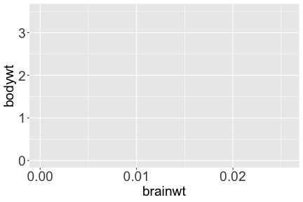
```

![](ggplot2_slides_files/figure-html/unnamed-chunk-8-1.png)

### `aes()`   _MAPS_   columns (variables!) onto the plot.
---

# Scatterplots in `ggplot2`

```r
ggplot(msleep_smol) + 
  (x = brainwt, y = bodywt)
```

```
## Error: <text>:2:15: unexpected ','
## 1: ggplot(msleep_smol) + 
## 2: (x = brainwt,
## ^
```

### Don't forget `aes()`!

---

# Scatterplots in `ggplot2`

```r
ggplot(msleep_smol) + 
  aes(x = brainwt, y = bodywt) + 
* geom_point()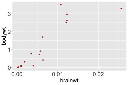
```

![](ggplot2_slides_files/figure-html/unnamed-chunk-10-1.png)

---

# Scatterplots in `ggplot2`

```r
ggplot(msleep_smol) + 
  aes(x = brainwt, y = bodywt) + 
* geom_point(color = "firebrick")
```

![](ggplot2_slides_files/figure-html/unnamed-chunk-11-1.png)

---

# Scatterplots in `ggplot2`

```r
ggplot(msleep_smol) + 
  aes(x = brainwt, y = bodywt) + 
* geom_point(color = "firebrick", size = 3)
```

![](ggplot2_slides_files/figure-html/unnamed-chunk-12-1.png)

---

# Plots can be saved just like variables

```r
sleep_scatter <- ggplot(msleep_smol) + 
 aes(x = brainwt, y = bodywt) + 
 geom_point(color = "firebrick", size = 3)

sleep_scatter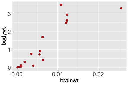
```

![](ggplot2_slides_files/figure-html/unnamed-chunk-13-1.png)

---

# Don't forget the _forward_ assignment operator

```r
ggplot(msleep_smol) + 
  aes(x = brainwt, y = bodywt) + 
  geom_point(color = "firebrick", size = 3) -> sleep_scatter

sleep_scatter
```

![](ggplot2_slides_files/figure-html/unnamed-chunk-14-1.png)

---

# Adding onto an existing plot

```r
ggplot(msleep_smol) + 
  aes(x = brainwt, y = bodywt) + 
  geom_point(color = "firebrick", size = 3) 
```

```r
ggplot(msleep_smol) + 
  aes(x = brainwt, y = bodywt) -> sleep_xy

sleep_xy + 
  geom_point(color = "firebrick", size = 3)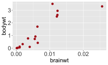
```

![](ggplot2_slides_files/figure-html/unnamed-chunk-16-1.png)

---

# Quick tangent: The plot theme

> The default theme is `theme_gray()` (`theme_grey()`)

.pull-left[

```r
sleep_scatter
```

![](ggplot2_slides_files/figure-html/unnamed-chunk-18-1.png)

```r
sleep_scatter + theme_classic()
```

![](ggplot2_slides_files/figure-html/unnamed-chunk-18-2.png)
]

.pull-left[

```r
sleep_scatter + theme_dark()
```

![](ggplot2_slides_files/figure-html/unnamed-chunk-19-1.png)

```r
sleep_scatter + theme_minimal()
```

![](ggplot2_slides_files/figure-html/unnamed-chunk-19-2.png)
]

---

# Adding on a theme

```r
ggplot(msleep_smol) + 
  aes(x = brainwt, y = bodywt) + 
  geom_point() + 
* theme_bw()
```

![](ggplot2_slides_files/figure-html/unnamed-chunk-20-1.png)

---

# Setting a theme for _all plots_

All plots created _after_ this line is run will use `theme_classic()`. All remaining plots in the slides will now use this theme as the new default.

```r
theme_set(theme_classic())
```

+ `get_help("theme_set")`
+ `get_help("theme_classic")`
+ All the built-in themes in action: https://spielmanlab.github.io/introverse/introverse_docs/ggplot2_theme_gray.html
+ Customizing themes: https://spielmanlab.github.io/introverse/articles/themes.html

---

# Histograms in `ggplot2`

### Goal: Visualize the distribution of all mammal times spent awake (`awake`)

### Step 1: Plan the plot *by hand*

---

# Histograms in `ggplot2`

```r
ggplot(msleep_smol)
```

![](ggplot2_slides_files/figure-html/unnamed-chunk-23-1.png)

---

# Histograms in `ggplot2`

```r
ggplot(msleep_smol) + 
* aes(x = awake)
```

![](ggplot2_slides_files/figure-html/unnamed-chunk-24-1.png)

---

# Histograms in `ggplot2`

```r
ggplot(msleep_smol) + 
  aes(x = awake) + 
* geom_histogram()
```

```
## `stat_bin()` using `bins = 30`. Pick better value with `binwidth`.
```

![](ggplot2_slides_files/figure-html/unnamed-chunk-25-1.png)

---

# Histograms in `ggplot2`

```r
ggplot(msleep_smol) + 
  aes(x = awake) + 
* geom_histogram(bins = 10)
```

![](ggplot2_slides_files/figure-html/unnamed-chunk-26-1.png)

### Use the argument `bins` to specify literally how many bins there should be
---

# Histograms in `ggplot2`

```r
ggplot(msleep_smol) + 
  aes(x = awake) + 
* geom_histogram(binwidth = 2)
```

![](ggplot2_slides_files/figure-html/unnamed-chunk-27-1.png)

### OR, use the argument `binwidth` to specify how wide the bins should be along the X-axis
---

# "Trial and error" to find the "right" binning

.pull-left[

```r
ggplot(msleep_smol) + 
  aes(x = awake) + 
* geom_histogram(bins = 2)
```

![](ggplot2_slides_files/figure-html/unnamed-chunk-28-1.png)
]

.pull-right[

```r
ggplot(msleep_smol) + 
  aes(x = awake) + 
* geom_histogram(bins = 30)
```

![](ggplot2_slides_files/figure-html/unnamed-chunk-29-1.png)
]

---

# Histograms in `ggplot2`

```r
ggplot(msleep_smol) + 
  aes(x = awake) + 
* geom_histogram(binwidth = 2, color = "dodgerblue")
```

![](ggplot2_slides_files/figure-html/unnamed-chunk-30-1.png)

---

# Histograms in `ggplot2`

```r
ggplot(msleep_smol) + 
  aes(x = awake) + 
* geom_histogram(binwidth = 2,
*                color = "dodgerblue")
```

![](ggplot2_slides_files/figure-html/unnamed-chunk-31-1.png)

### When code gets long, separate onto multiple lines for clarity. _YOU WILL BE GRADED ON THIS!!!!_
---

# Histograms in `ggplot2`

```r
ggplot(msleep_smol) + 
  aes(x = awake) + 
  geom_histogram(binwidth = 2,   
                 color = "dodgerblue",
*                fill = "orange")
```

![](ggplot2_slides_files/figure-html/unnamed-chunk-32-1.png)

---

# Histograms in `ggplot2`

```r
ggplot(msleep_smol) + 
  aes(x = awake) + 
  geom_histogram(binwidth = 2,   
                 color = "dodgerblue",
                 fill = "orange",
*                size = 3)
```

![](ggplot2_slides_files/figure-html/unnamed-chunk-33-1.png)
 
**This is _pretty ugly_, but now you've learned about `size`!**
---

# COMMENT COMMENT COMMENT COMMENT

```r
ggplot(msleep_smol) + 
  # specify x on the x-axis 
  aes(x = awake) + 
  geom_histogram(binwidth = 2, # use binwidth of 2  
                 # outline the histogram in blue
                 color = "dodgerblue", 
                 # fill the bars with orange 
                 fill = "orange", 
                 # increase width of histogram lines    
                 size = 3)   
```

![](ggplot2_slides_files/figure-html/unnamed-chunk-34-1.png)

---

# Density plots in `ggplot2`

### Goal: Visualize the distribution of all mammal times spent awake (`awake`) for each vore

### Step 1: Draw it by hand

---

# Density plots in `ggplot2`

```r
ggplot(msleep_smol) + 
  aes(x = awake) + 
* geom_density()
```

![](ggplot2_slides_files/figure-html/unnamed-chunk-35-1.png)

---

# Density plots in `ggplot2`

```r
ggplot(msleep_smol) + 
  aes(x = awake) + 
* geom_density(fill = "cornflowerblue",
*              color = "chartreuse",
*              size = 4)
```

![](ggplot2_slides_files/figure-html/unnamed-chunk-36-1.png)

### Again, kinda ugly, but look how easy that was to make!!

---

# What if we wanted to show *all vores* separately?

### Conceptualize by hand:

---
# Density plots in `ggplot2`

```r
ggplot(msleep_smol) +  
* aes(x = awake, fill = vore) +
  geom_density()
```

![](ggplot2_slides_files/figure-html/unnamed-chunk-37-1.png)

### We need to make the density plots _transparent_.
---

# Density plots in `ggplot2`

```r
ggplot(msleep_smol) +  
* aes(x = awake, fill = vore) +
* geom_density(alpha = 0.5)
```

![](ggplot2_slides_files/figure-html/unnamed-chunk-38-1.png)

+ `alpha` is NOT a variable, so it does NOT belong in `aes()`. It is a visual aspect of the *density plot*, so we provide the argument to `geom_density()`
  + `alpha = 1`: Completely transparent. 
  + `alpha = 0`: Completely opaque

---

# Density plots in `ggplot2`

```r
ggplot(msleep_smol) +  
  aes(x = awake, 
*     fill = vore,
*     color = vore) +
  geom_density(alpha = 0.5) 
```

![](ggplot2_slides_files/figure-html/unnamed-chunk-39-1.png)

### We will learn how to customize these colors next week

---

# Boxplots in `ggplot2`

### Goal: Visualize the distribution of all mammal times spent awake (`awake`) for each vore

### Step 1:

---

# Boxplots in `ggplot2`

```r
ggplot(msleep_smol) + 
* aes(x = vore, y = awake)
```

![](ggplot2_slides_files/figure-html/unnamed-chunk-40-1.png)
---

# Boxplots in `ggplot2`

```r
ggplot(msleep_smol) + 
  aes(x = vore, y = awake) +
* geom_boxplot()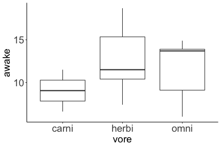
```

![](ggplot2_slides_files/figure-html/unnamed-chunk-41-1.png)
---

# Boxplots in `ggplot2`

```r
ggplot(msleep_smol) + 
  aes(x = vore, y = awake) +
* geom_boxplot(color = "deeppink",
*              fill  = "goldenrod1")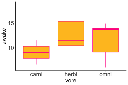
```

![](ggplot2_slides_files/figure-html/unnamed-chunk-42-1.png)
--

### What if we want a separate fill _for each vore_?

---

# Boxplots in `ggplot2`

```r
ggplot(msleep_smol) + 
* aes(x = vore, y = awake, fill = vore) +
  geom_boxplot()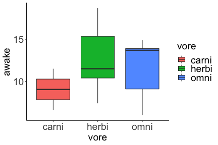
```

![](ggplot2_slides_files/figure-html/unnamed-chunk-43-1.png)

---

# Violin plots in `ggplot2`

.pull-left[

```r
ggplot(msleep_smol) + 
  aes(x = vore, y = awake) +  
* geom_violin()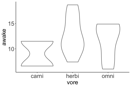
```

![](ggplot2_slides_files/figure-html/unnamed-chunk-44-1.png)
]

.pull-right[

```r
ggplot(msleep_smol) + 
  aes(x = vore, 
      y = awake, 
*     fill = vore) +
  geom_violin() 
```

![](ggplot2_slides_files/figure-html/unnamed-chunk-45-1.png)
]

---

# Strip/jitter plots in `ggplot2`

```r
ggplot(msleep_smol) + 
  aes(x = vore, y = awake) +
  # size = 2 to see more easily in slides
* geom_jitter(size = 2)
```

![](ggplot2_slides_files/figure-html/unnamed-chunk-46-1.png)

---

# Strip/jitter plots in `ggplot2`

```r
ggplot(msleep_smol) + 
  aes(x = vore, y = awake) +  
* geom_jitter(width = 0.2,
              size  = 2)
```

![](ggplot2_slides_files/figure-html/unnamed-chunk-47-1.png)

### Usually need to pick a width between 0.1 - 0.3, *in my opinion*

---
# Strip/jitter plots in `ggplot2`

```r
ggplot(msleep_smol) + 
  # COLOR, NOT FILL!! These are points
  aes(x = vore, 
      y = awake, 
*     color = vore) +
  geom_jitter(width = 0.2, size = 2) 
```

![](ggplot2_slides_files/figure-html/unnamed-chunk-48-1.png)
 
**Did you notice the points were placed little differently each plot version?**
---

# Other types of points

+ Any time you use `geom_point()` or `geom_jitter()` you can specify a different point!
+ _Point shapes 21-25 have a color and a fill_

---

# Example of shape 21

```r
ggplot(msleep_smol) +
  aes(x = vore, 
      y = awake, 
*     fill = vore) +
  geom_jitter(width = 0.2, 
              size = 4,
*             color = "black",
*             shape = 21)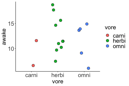
```

![](ggplot2_slides_files/figure-html/unnamed-chunk-50-1.png)

---

# Barplots in `ggplot2`

### Goal: How many of each vore are there?

> Note: There are many ways to make barplots. Today we will learn how to make barplots specifically to show _amount of a categorical variable._

### Step 1:

---

# Barplots in `ggplot2`

```r
ggplot(msleep_smol) +
  aes(x = vore) + 
* geom_bar()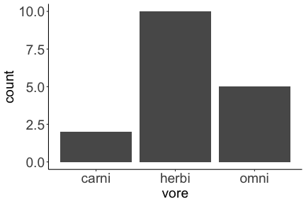
```

![](ggplot2_slides_files/figure-html/unnamed-chunk-51-1.png)

---
# Barplots in `ggplot2`

```r
ggplot(msleep_smol) +
  aes(x = vore) + 
* geom_bar(fill = "blueviolet")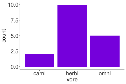
```

![](ggplot2_slides_files/figure-html/unnamed-chunk-52-1.png)
---
# Barplots in `ggplot2`

```r
ggplot(msleep_smol) +
  aes(x = vore) + 
* geom_bar(fill = "blueviolet",
*          color = "black", size = 2)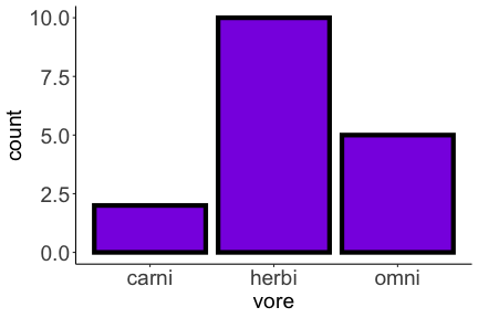
```

![](ggplot2_slides_files/figure-html/unnamed-chunk-53-1.png)
---

# Barplots in `ggplot2`

```r
ggplot(msleep_smol) +
  aes(x = vore,
*     fill = vore) +
  geom_bar()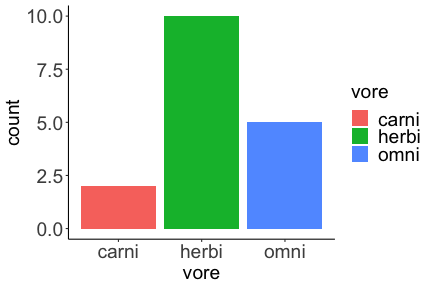 
```

![](ggplot2_slides_files/figure-html/unnamed-chunk-54-1.png)
---

# Barplots in `ggplot2`

```r
ggplot(msleep_smol) +
  aes(x = vore,
      fill = vore) +  
* geom_bar(color = "black")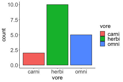
```

![](ggplot2_slides_files/figure-html/unnamed-chunk-55-1.png)
---

# Barplots in `ggplot2`

```r
ggplot(msleep_smol) +
  aes(x = vore,
*     fill = conservation) +
  geom_bar() 
```

![](ggplot2_slides_files/figure-html/unnamed-chunk-56-1.png)

---

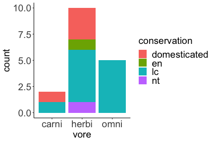# Barplots in `ggplot2`

```r
ggplot(msleep_smol) +
  aes(x = vore,
      fill = conservation) + 
* geom_bar(position = position_dodge())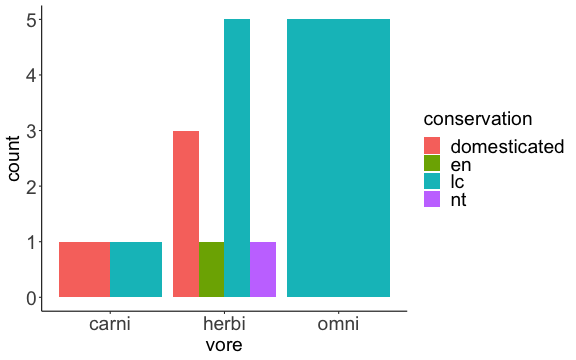
```

![](ggplot2_slides_files/figure-html/unnamed-chunk-57-1.png)

---

# Barplots in `ggplot2`

```r
ggplot(msleep_smol) +
  aes(x = vore,
      fill = conservation) + 
* geom_bar(position = position_dodge(preserve="single"))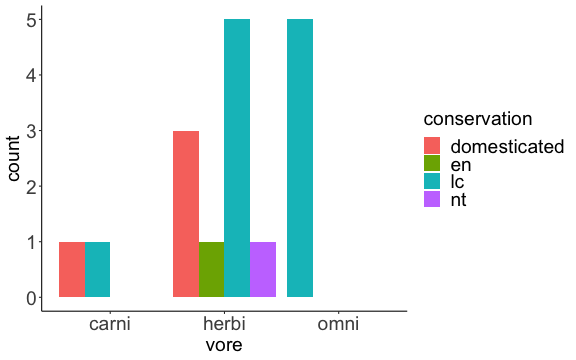
```

![](ggplot2_slides_files/figure-html/unnamed-chunk-58-1.png)

---

# Barplots in `ggplot2`

.pull-left[

```r
ggplot(msleep_smol) +
  aes(x = vore,
      fill = conservation) +  
  geom_bar() 
```

![](ggplot2_slides_files/figure-html/unnamed-chunk-59-1.png)
]

.pull-right[

```r
ggplot(msleep_smol) +
  aes(x = conservation,
      fill = vore) +  
  geom_bar()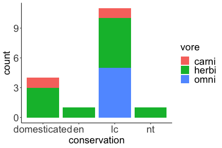 
```

![](ggplot2_slides_files/figure-html/unnamed-chunk-60-1.png)
]

---

# Barplots in `ggplot2`

```r
ggplot(msleep_smol) +
  aes(x = vore,
      fill = order) +  
  geom_bar()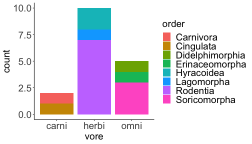 
```

![](ggplot2_slides_files/figure-html/unnamed-chunk-61-1.png)

### My first impression of this plot is _feeling overwhelmed_.

---

# Labeling your plots

```r
ggplot(msleep_smol) +
  aes(x = vore) +  
  geom_bar()  + 
* labs(x = "X-axis label",
*      y = "Y-axis label",
*      title = "Plot title",
*      subtitle = "In case you wanted a subtitle",
*      caption = "Would you like a caption?")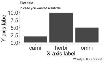
```

![](ggplot2_slides_files/figure-html/unnamed-chunk-62-1.png)

Always make sure your x and y axes are professionally labeled (*no underscores!*). Title, subtitle, caption are optional to include.

---

# Plots we can make!

![](ggplot2_slides_files/figure-html/unnamed-chunk-64-1.png)![](ggplot2_slides_files/figure-html/unnamed-chunk-64-2.png)

---

# Adding panels ("facets") to plots

```r
ggplot(msleep_smol, aes(x = awake)) + 
  geom_histogram(binwidth = 2, 
                 color = "black", 
                 fill = "firebrick2")
```

![](ggplot2_slides_files/figure-html/unnamed-chunk-66-1.png)

### What if we want a separate histogram for each `vore`?

---

# This is a bad idea.

```r
ggplot(msleep_smol, aes(x = awake, fill = vore)) + 
  geom_histogram(binwidth = 2, 
                 color = "black")
```

![](ggplot2_slides_files/figure-html/unnamed-chunk-67-1.png)

---

# Adding panels ("facets") to plots

```r
ggplot(msleep_smol, aes(x = awake)) + 
  geom_histogram(binwidth = 2, # may need to tweak again!
                 color = "black", 
                 fill = "firebrick2")  +
* facet_wrap( vars(vore) )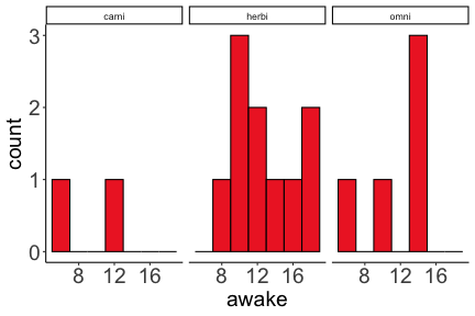
```

![](ggplot2_slides_files/figure-html/unnamed-chunk-68-1.png)
 
**Faceting is the _ONLY TIME_ we do not use `aes()` to refer to a column!!! We use `vars()` when faceting.**

---

# Adding panels ("facets") to plots

```r
ggplot(msleep_smol, aes(x = awake)) + 
  geom_histogram(binwidth = 2, # may need to tweak again!
                 color = "black", 
                 fill = "firebrick2")  +
  # you get to choose which is row and which is column
* facet_grid( rows = vars(vore),
*             cols = vars(conservation) )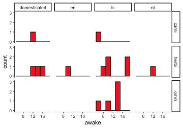
```

![](ggplot2_slides_files/figure-html/unnamed-chunk-70-1.png)

**Use `facet_grid()` to make a panel grid across 2 variables. This plot is _pretty bad_, but it teaches `facet_grid()`!**