Inclass exercises solutions, Day 9
Follow this link for day 9 materials and notes
ANOVA
Using the built-in dataset PlantGrowth, run an ANOVA to determine if plant weight differs across treatments.
Solution
> head(PlantGrowth)
  weight group
1   4.17  ctrl
2   5.58  ctrl
3   5.18  ctrl
4   6.11  ctrl
5   4.50  ctrl
6   4.61  ctrl

> fit <- aov(weight ~ group, data = PlantGrowth)
> summary(fit)
            Df Sum Sq Mean Sq F value Pr(>F)
group        2  3.766  1.8832   4.846 0.0159 *
Residuals   27 10.492  0.3886
---
Signif. codes:  0 ‘***’ 0.001 ‘**’ 0.01 ‘*’ 0.05 ‘.’ 0.1 ‘ ’ 1

### For demonstrative purposes, run a Tukey-Kramer test. Not necessary for every ANOVA!
> TukeyHSD(fit)
  Tukey multiple comparisons of means
    95% family-wise confidence level

Fit: aov(formula = weight ~ group, data = PlantGrowth)

$group
            diff        lwr       upr     p adj
trt1-ctrl -0.371 -1.0622161 0.3202161 0.3908711
trt2-ctrl  0.494 -0.1972161 1.1852161 0.1979960
trt2-trt1  0.865  0.1737839 1.5562161 0.0120064
Our null for the ANOVA is that all plant treatments have the same mean weight. Our alternative hypothesis is that at least one group has a different weight. ANOVA gives F = 4.806 with P=0.0159 which is significant at alpha = 0.05. We reject the null hypothesis and find evidence that at least one plant group has a different mean weight.
A post-doc Tukey test shows that trt1 and trt2 have significantly different weights (P=0.012) but that there is no evidence for weight differences for other group comparisons.
Pearson’s Correlation
Using the dataset wine.csv, run a correlation test to determine the strength and magnitude of the relationship between flavanoid and total phenol content across all wine cultivars.
Solution
> wine <- read.csv("wine.csv")
> head(wine)
  Cultivar Alcohol MalicAcid  Ash Magnesium TotalPhenol Flavanoids
1        1   14.23      1.71 2.43       127        2.80       3.06
2        1   13.20      1.78 2.14       100        2.65       2.76
3        1   13.16      2.36 2.67       101        2.80       3.24
4        1   14.37      1.95 2.50       113        3.85       3.49
5        1   13.24      2.59 2.87       118        2.80       2.69
6        1   14.20      1.76 2.45       112        3.27       3.39
  NonflavPhenols Color
1           0.28  5.64
2           0.26  4.38
3           0.30  5.68
4           0.24  7.80
5           0.39  4.32
6           0.34  6.75

## Check linearity
> ggplot(wine,aes(x = Flavanoids, y = TotalPhenol))+geom_point()

## Run correlation
> cor.test(wine$Flavanoids, wine$TotalPhenol)

	Pearson's product-moment correlation

data:  wine$Flavanoids and wine$TotalPhenol
t = 22.824, df = 176, p-value < 2.2e-16
alternative hypothesis: true correlation is not equal to 0
95 percent confidence interval:
 0.8220088 0.8975164
sample estimates:
      cor
0.8645635

The Pearson correlation between Flavanoids and TotalPhenol is R=0.86, and is significantly different from 0 (P<2.2e-16). Therefore these two quantities have strong and positive linear relationship.
Spearman’s Correlation
Using the ggplot2 dataset diamonds (you can access it like any built-in dataset if ggplot2 is loaded), run a non-parametric correlation test between diamond carat and price, specifically for diamonds with quality “Good”.
Solutions
> head(diamonds)
# A tibble: 6 x 10
  carat       cut color clarity depth table price     x     y     z
1  0.23     Ideal     E     SI2  61.5    55   326  3.95  3.98  2.43
2  0.21   Premium     E     SI1  59.8    61   326  3.89  3.84  2.31
3  0.23      Good     E     VS1  56.9    65   327  4.05  4.07  2.31
4  0.29   Premium     I     VS2  62.4    58   334  4.20  4.23  2.63
5  0.31      Good     J     SI2  63.3    58   335  4.34  4.35  2.75
6  0.24 Very Good     J    VVS2  62.8    57   336  3.94  3.96  2.48

#### Subset for correlation
diamonds %>% filter(cut == "Good") -> good

## Check linearity
> ggplot(good,aes(x = price, y = carat))+geom_point()

## Run correlation
> cor.test(good$price, good$carat, method = "spearman")
	Spearman's rank correlation rho

data:  good$price and good$carat
S = 787830000, p-value < 2.2e-16
alternative hypothesis: true rho is not equal to 0
sample estimates:
      rho
0.9599684 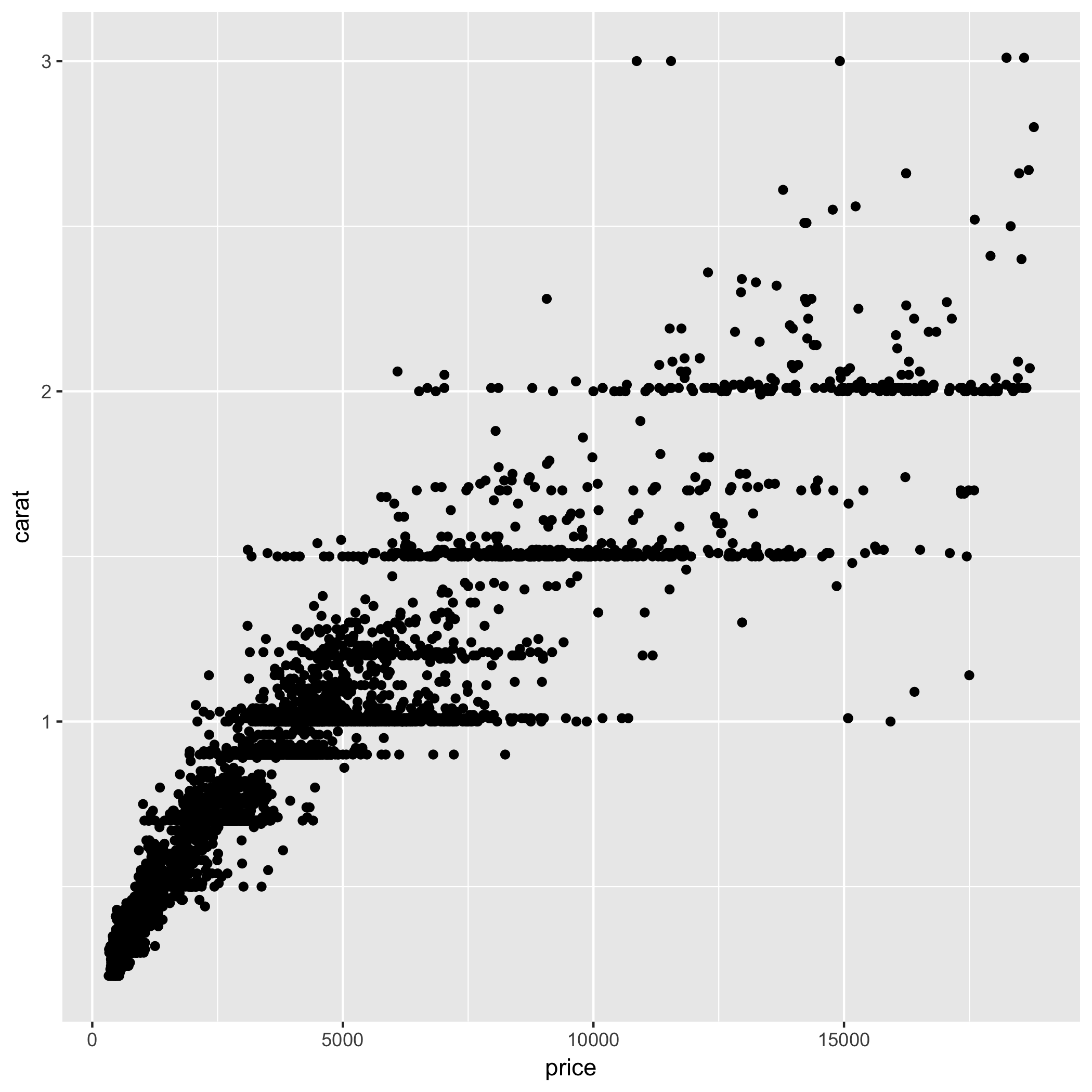
Diamond carat and price are not linearly related, as seen through plotting, so we must use a nonparametric correlation. The Spearman correlation between Flavanoids and TotalPhenol is R=0.96, and is significantly different from 0 (P<2.2e-16). Therefore these two quantities have strong and positive (but not linear!) relationship.
Regression
Using the dataset wine.csv, construct a linear model that can predict the amount of Flavanoids from the amount of non-flavanoid phenols (NonflavPhenols) across all wine cultivars. Then, predict the Flavanoid content for a wine with non-flavanoid phenols of 0.12.
## Check linearity with response on y axis
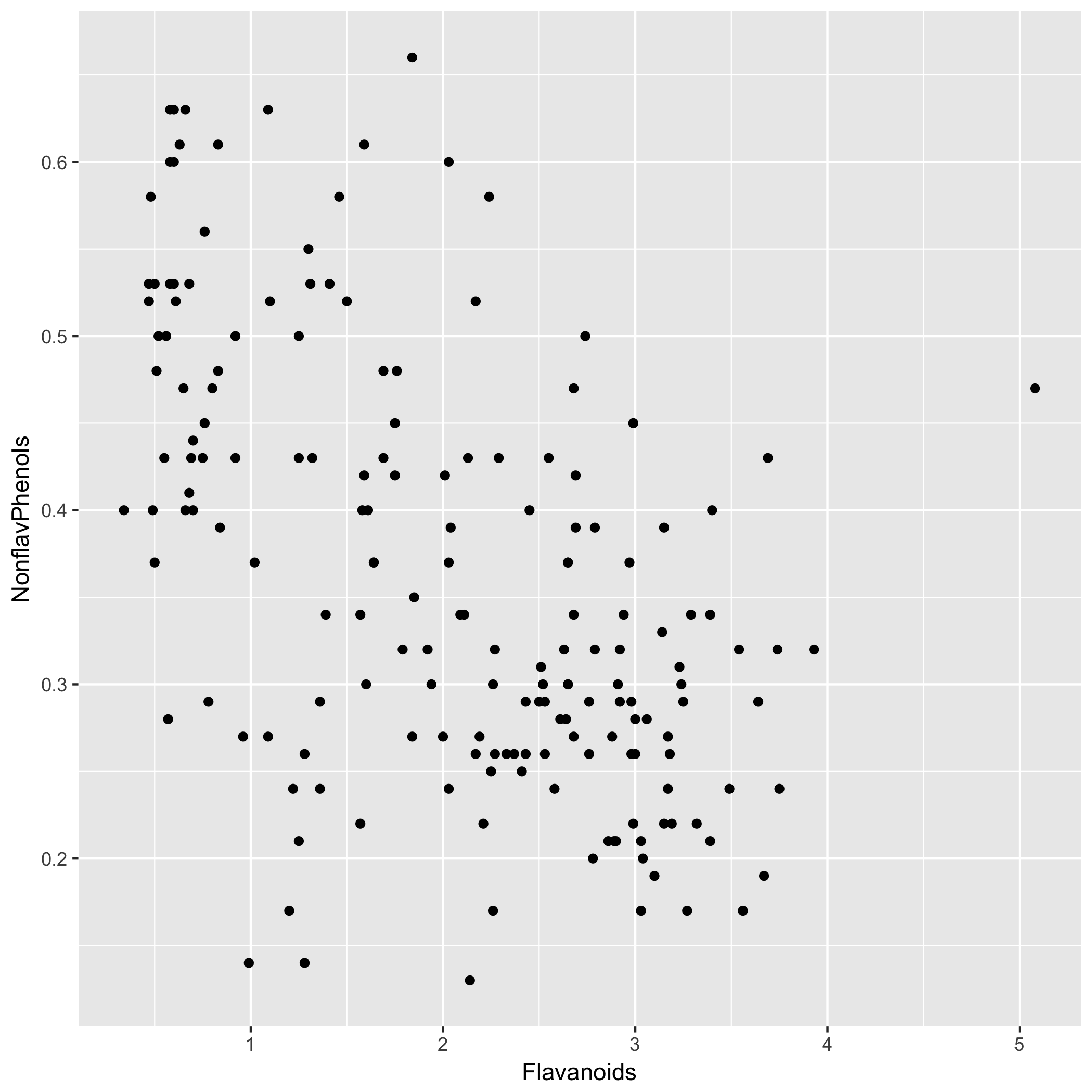
> ggplot(wine,aes(x = Flavanoids, y = NonflavPhenols))+geom_point()
## Fit model
> fit <- lm(NonflavPhenols ~ Flavanoids, data = wine)
> summary(fit)
Call:
lm(formula = NonflavPhenols ~ Flavanoids, data = wine)
Residuals:
Min 1Q Median 3Q Max
-0.29151 -0.06631 -0.01409 0.06859 0.31261
Coefficients:
Estimate Std. Error t value Pr(>|t|)
(Intercept) 0.497855 0.017897 27.817 < 2e-16 ***
Flavanoids -0.067020 0.007917 -8.465 9.74e-15 ***
---
Signif. codes: 0 ‘***’ 0.001 ‘**’ 0.01 ‘*’ 0.05 ‘.’ 0.1 ‘ ’ 1
Residual standard error: 0.1052 on 176 degrees of freedom
Multiple R-squared: 0.2893, Adjusted R-squared: 0.2853
F-statistic: 71.66 on 1 and 176 DF, p-value: 9.739e-150.9599684
### Note the broom package!
> tidy(fit)
term estimate std.error statistic p.value
1 (Intercept) 0.49785537 0.017897438 27.81713 2.490523e-66
2 Flavanoids -0.06701989 0.007917322 -8.46497 9.739231e-15
> glance(fit)
r.squared adj.r.squared sigma statistic p.value df logLik
1 0.289336 0.2852981 0.1052129 71.65571 9.739231e-15 2 149.2495
AIC BIC deviance df.residual
1 -292.4991 -282.9537 1.948277 176
Check linearity:
Add regression line:
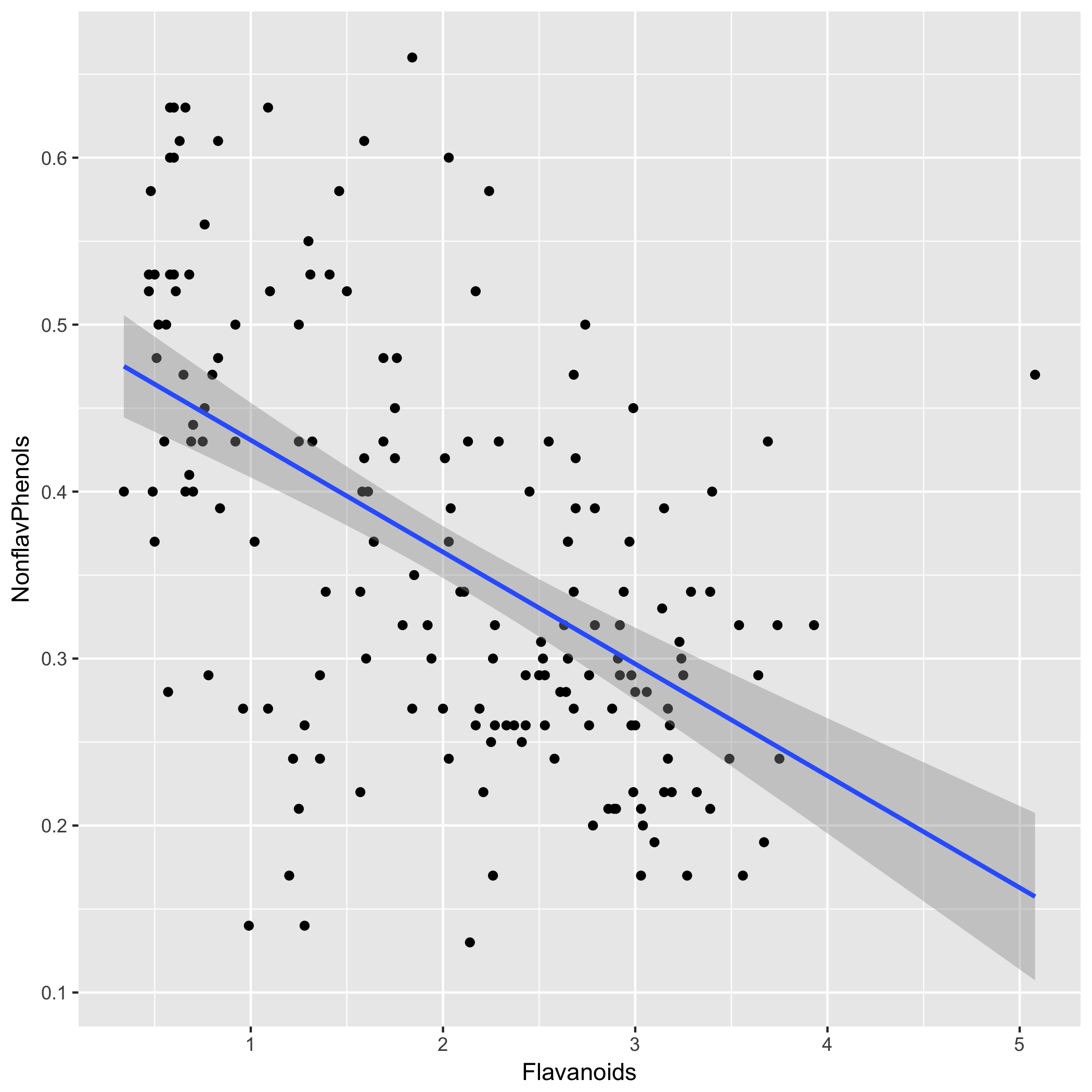
Our model shows a moderate but significant relationship between flavanoids and non-flavanoid phenols. Our model’s (P=9.74e-15) is highly significant and indicates that flavanoid content can explain ~29% of variation in non-flavanoid phenols. Therefore, the model does not explain the majority of variation in non-flavanoid phenols.
The flavanoid coefficient is -0.067 (P=9.74e-15), meaning that for every unit increase in flavanoid content, we expect non-flavanoid phenols to decrease by 0.067 units on average. The intercept is 0.498 (P=2.49e-66), so wine with 0 flavanoid content is expected to contain 0.497 units of non-flavanoid phenols, although this quantity is probably not meaningful in the context of actual wine.