Inclass exercises solutions, Day III
Binomial test
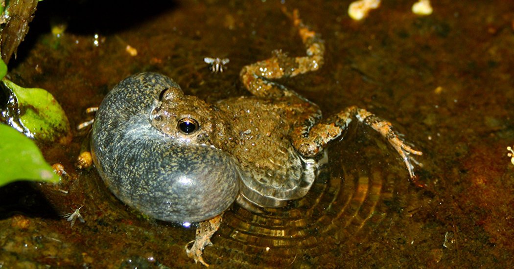
Tungara frogs (pictured below) have been heavily studied as a model organism for “female mate choice”. These frogs emit mating calls which are either “whines” or “whine-chuck”, where “chuck” noises are tacked on to the whine to create a longer, more robust mating call.
Researchers wanted to test whether mating calls with chucks were more likely to attract females. In an experiment, researchers placed female frogs in the middle of a room and played different male mating calls (whine or whine-chuck) on either end of the room, allowing female frogs hop towards their preferred noise. Researchers randomly selected 15 non-gravid female tungara frogs to test. One at a time, each female frog was given the opportunity to choose between two vocalizations (without seeing a male): whine and whine-chuck. The noise the female walks towards indicates her mate choice. Ultimately, they found that 2 female frogs preferred whine, and 13 female frogs preferred whine-chuck.
Conduct a binomial test to ask if females showed a preference for whine-chunk. Take the following steps:
- Understand why the binomial test is applicable here
- Determine the appropriate null probability of success
- Estimate the probability of success from the data, including the estimate and standard error
- State the null, alternative hypotheses
- Conduct the test
- Report results, conclusions
Solution
Ho: Female tungara frogs have no preference for whine or whine-chuck (p=0.5)
Ha: Female tungara frogs have a preference for whine or whine-chuck (p!=0.5)
n <- 15
k <- 13 ## k<-2 would also work
pnull <- 0.5

## Estimate probability of success
p.hat <- k/n # Evaluates to 0.8666667
## Estimate SE
p.hat_se <- sqrt(p.hat*(1-p.hat)/n) # Evaluates to 0.08777075


## Perform binomial test
binom.test(k, n, pnull)
#
#	Exact binomial test
#
#data:  k and n
#number of successes = 13, number of trials = 15, p-value = 0.007385
#alternative hypothesis: true probability of success is not equal to 0.5
#95 percent confidence interval:
# 0.5953973 0.9834241
#sample estimates:
#probability of success
#             0.8666667
Results and conclusions: Our P=0.007385 is less than . We reject the null hypothesis and conclude that there is evidence that females display a preference for whine or whine-chuck. Our estimated probability of success is 0.87 with SE = 0.088, which means we have evidence for a whine-chuck preference in non-gravid female tungara frogs.
goodness-of-fit test
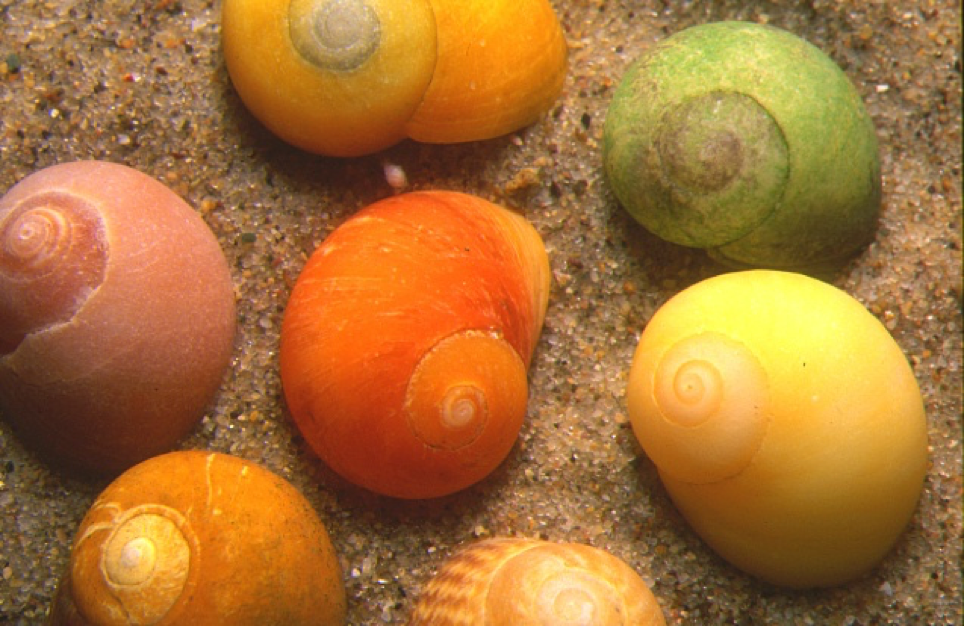
Periwinkles, small species of sea snail (pictured below) eat seaweed. Researchers want to know if periwinkles have a preference for different seaweed plants.
In one tidal pool, researchers count the number of periwinkles found feeding on four different kinds of seaweed: spiral wrack, bladder wrack, toothed wrack, and knotted wrack. Researchers also measured the relative frequencies of these four seaweed species in this environement. A table giving the number of periwinkles eating on, and the frequency of different seaweeds is below:
| Seaweed | Seaweed frequency | Number of perwinkles eating it |
|---|---|---|
| Spiral wrack | 10% | 9 |
| Bladder wrack | 25% | 28 |
| Toothed wrack | 15% | 19 |
| Knotted wrack | 50% | 64 |
Conduct a goodness-of-fit test to ask if periwinkles feed on seaweed with no preference for species. Take the following steps:
- Understand why the goodness-of-fit test is applicable here
- Determine the appropriate null frequencies
- State the null, alternative hypotheses
- Conduct the test
- Report results, conclusions
Solution
Ho: Periwinkles have no preference for seaweed species and feed on spiral:bladder:toothed:knotted with a null frequency distribution of 0.1:0.25:0.15:0.5.
Ha: Periwinkles have a preference for seaweed species and feed on spiral:bladder:toothed:knotted with a frequency distribution that differs from 0.1:0.25:0.15:0.5.
observed <- c(9, 28, 19, 64)
expected <- c(0.1, 0.25, 0.15, 0.5)

chisq.test(observed, p = expected)
#
#	Chi-squared test for given probabilities
#
#data:  observed
#X-squared = 1.2056, df = 3, p-value = 0.7517
Results and conclusions: Our P=0.75 is greater than . We fail to reject the null hypothesis. We conclude that there is no evidence that periwinkles have a preference for seaweed species. In other words, we have no evidence that feeding on spiral:bladder:toothed:knotted differs from 0.1:0.25:0.15:0.5.
Contingency table analysis
In 1999, Researchers studied the prevalence of Hepatitis C (HCV) in Americans to determine if there is an association between the number of sexual partners an individual has had and the presence of HCV. They took a random sample of 11,106 records from a National Health Survey to assess this association. Their data is found in the file hcv_partners.csv.
Conduct a contingency table test to ask if HCV prevalence is associated with having many (>=10) or few (<10) partners. Take the following steps:
- Read in and examine the data
- Figure out how to create your contingency table from the dataframe (hint: you will need
dplyrfunctions includingfilter()andtally(), and if you recall how to useifelse()this may be of interest as well)- Variable 1: Has HCV (1) or not (0)
- Variable 2: Has had < 10 partners or >=10 partners
- State the null, alternative hypotheses
- Create your contingency table in R
- Conduct the test
- Report results, conclusions
Ho: There is no association between HCV and have many (>=10) or few (<10) sexual partners.
Ha: There is an association between HCV and have many (>=10) or few (<10) sexual partners.
library(tidyverse)
hcv.data <- read.csv("hcv_partners.csv")

### Create the table
topleft <- hcv.data %>% filter(HCV == 1, partners >=10) %>% tally()
topright <- hcv.data %>% filter(HCV == 0, partners >=10) %>% tally()
bottomleft <- hcv.data %>% filter(HCV == 1, partners <10) %>% tally()
bottomright <- hcv.data %>% filter(HCV == 0, partners <10) %>% tally()
hcv.table <- rbind(c(topleft$n, topright$n), c(bottomleft$n,  bottomright$n))
#hcv.table
#     [,1] [,2]
#[1,]  166 2587
#[2,]   75 8278

### Perform test
chisq.test(hcv.table)
#
#	Pearson's Chi-squared test with Yates' continuity correction
#
#data:  hcv.table
#X-squared = 254.46, df = 1, p-value < 2.2e-16

### Compute OR
OR <- (166*8278)/(75*2587) ## Evaluates to 7.082324
Results and conclusions: Our P<2.2e-16 (note: this is as low as R can go!) is less than . We reject the null hypothesis and we conclude that there is an association between having many partners and having HCV. Further, we can conclude that individuals with many sexual partners have 7.08 times the odds of having HCV compared to individuals with few partners.